

1 Sequencing system migration after an acquisition
A mid-market acquisition can leave a buyer with several systems to join, including the customer master, the product and price catalogue, order management, billing, payments, the general ledger and the service desk. The constructed programme in this paper uses these seven systems to examine the trade-off between temporary interfaces, conversion defects and concentrated cutover risk. A live programme would need its own application inventory, transition architecture and calendar before these costs could be estimated. The research question is which migration order minimises transaction errors and customer-service interruption under stated assumptions.
The framework has three assumed mechanisms. Interfaces between different platforms accumulate errors and outage exposure while their endpoints remain separated. Conversion defects depend on upstream readiness, learning, concurrency and overlapping hypercare. Each cutover creates an exposure profile, with a conditional extension if the wave fails. The calculation compares 5,040 strict seven-wave orders and 47,293 ordered plans in which two or more systems may share a wave. The same objective and base inputs apply to every candidate. A separate relative-readiness constraint illustrates how a dated operating requirement can alter the feasible set.
Earlier MatchPoint Insights address continuity tolerances, dependency mapping, migration waves, cutover gates and customer consequences. The ERP and data-migration framework includes a migration-wave matrix and an interface dependency graph; the technology-stack framework includes migration estimates and customer revenue-at-risk. [18, 19] This paper examines a narrower decision within those frameworks through an explicitly authored seven-system numerical comparison of orders and shared-wave plans. The analysis reports conditional model outcomes and a proposed evidence design. In the constructed programme the lowest-loss order, PC > OM > CM > BI > PA > GL > CS, has an expected loss of USD 300.44 thousand, against USD 386.58 thousand for an order chosen at random.
2 Outcomes and valuation of operational exposure
The transaction-error outcome counts erroneous processing events associated with a temporary interface or a converted record under the assumed mechanism. An event can concern an order, invoice, payment application, ledger posting or service case. These counts can include several processing events for one commercial transaction. They are not counts of unique customers, legal invoices or independently verified incidents. The model reports expected counts conditional on its inputs; a practical implementation needs an event taxonomy and a rule for attributing and deduplicating observed errors.
Interruption is measured as customer-event exposure-hours. Within one wave, systems start their cutovers simultaneously. An integral counts the expected customer share exposed to at least one unavailable system at each point in time, using authored independent exposure indicators and each system's duration. The resulting wave totals are then added across waves and bridge flows. That final sum can count the same customer-clock hour under more than one distinct event. It is an exposure index, and is not a deduplicated whole-programme outage measure. A buyer seeking unique interruption hours would need joint customer-level timelines or a separately justified dependence model.
The loss objective assigns USD 45 of repair cost to each erroneous transaction event. It then applies a weight of 0.003 departure equivalents per visibility-weighted error and 0.00002 per customer-event exposure-hour, valued at USD 15,000 annual gross revenue per departure equivalent. These are author-selected valuation weights. They are not estimated departure probabilities, and repeated exposure is not converted into a claim about unique lost customers. The objective combines error-repair expenditure with a gross-revenue-equivalent index. Finance would need margins, timing, recoveries, customer responses and discounting to translate it into a cash-flow or valuation effect.
3 Evidence from public migration failures
The Prudential Regulation Authority's final notice to the former chief information officer of TSB Bank records that the bank had about 5.2 million customers and decided in December 2015 to migrate to a new platform. The migration was to be a predominantly single main event, with some functions, including the faster payments system, the mobile app and cash machines, moved earlier through governed transition events from 2017. The main event took place over the weekend of 20 to 22 April 2018. The notice states that the data migration itself was successful, yet online, telephone and mobile banking and branch technology failed, with all 550 branches affected, and that rollback after the event was essentially impossible. [1]
The Financial Conduct Authority's announcement adds that the FCA and the PRA together fined the bank GBP 48.65 million in December 2022, of which GBP 29.75 million was the FCA penalty and GBP 18.9 million the PRA penalty, that business as usual returned in December 2018 and that GBP 32.7 million was paid in redress. It names the failure to organise and control the migration programme and to manage the risks of outsourcing to a critical supplier. [2] The sanction in the notice is against an individual senior manager for outsourcing oversight. It does not find that a single-event approach caused the failure, and a bank with millions of retail customers differs in scale from a mid-market business. TSB therefore shows the shape and size of customer-visible interruption. It does not test an order.
Revlon's 2018 annual report describes service-level disruption following the February 2018 SAP launch at its Oxford, North Carolina manufacturing facility. The company estimated that the launch left it unable to fulfil shipments representing approximately USD 64 million of net sales during 2018 and resulted in USD 53.6 million of incremental charges in 2018, mainly for remedial customer-service actions. It reported a material weakness in internal control over financial reporting and stated that the Oxford facility was operating at pre-SAP levels at 31 December 2018 while retail-partner inventories were still being replenished. [3] These are issuer-reported estimates and control findings from a U.S. implementation. The cited passages provide no comparison between acquisition-migration orders and supply no rate for this constructed model. Table 1 separates the reported mechanism from that identification limit.
| Case | What the source establishes | What it does not establish |
|---|---|---|
| TSB main migration event, April 2018 | Single main event after earlier governed transitions; data migrated but services failed across all branches; rollback not practicable after the event [1] | That the single-event design caused the failure; any rate applicable to a mid-market buyer |
| TSB sanctions, December 2022 | Joint fine of GBP 48.65 million; GBP 32.7 million redress; failures of programme control and outsourcing risk management [2] | That a different order would have avoided the failure |
| Revlon enterprise-system launch, 2018 | Issuer-estimated unfulfilled shipments representing approximately USD 64 million of 2018 net sales; USD 53.6 million of 2018 incremental charges; material weakness in internal control over financial reporting [3] | That the launch was an acquisition integration; the order of any workstream |
Basis: the cited regulatory notices and issuer filing. The cases describe disruption mechanisms and scale; no model rate is calibrated from them. [1, 2, 3]
4 Integration research and prior sequencing approaches
Henningsson, Yetton and Wynne reviewed 70 articles published between 1989 and 2016 on information-system integration in mergers and acquisitions, coding 53 dependent and 195 independent variables. Their accepted manuscript discusses absorption, co-existence, best-of-breed and renewal, as well as interim integration methods adopted under legal and regulatory time pressure. It also describes a hospital-merger example in which patient administration was integrated first for operational reasons and financial and managerial systems followed. [4] These selected findings show that context and phasing already form part of the integration literature. The present calculation applies dependency and sequencing ideas to one authored network; it provides no general ranking of real acquisition programmes.
Tanriverdi and Uysal's published abstract reports a sample of 141 acquisitions by 86 Fortune 1000 firms. Higher cross-business IT integration capability is associated with positive and significant cumulative abnormal announcement returns and higher long-run abnormal operating performance. The larger complementary cross-industry advantage concerns long-run operating performance. [5] This abstract-level evidence concerns large acquirers and capability-value associations. It provides contextual motivation for this paper; no workstream-order effect or numerical calibration is taken from it.
Homburg and Bucerius's published abstract reports an empirical sample of 232 horizontal mergers and acquisitions. It describes integration speed as beneficial when external relatedness is low and internal relatedness is high, and detrimental in the opposite configuration. [6] This is abstract-level contextual evidence. The present paper treats spacing as a conditional model input to test; no bridge error rate, conversion rate or numerical migration order is calibrated from either published abstract.
5 E-invoicing scope and the readiness calendar
The UAE timetable is set out in Ministerial Decision 244 of 2025 as amended by Decision 66 of 2026. For a Person subject to the system with Revenue equal to or above AED 50 million, the accredited-service-provider appointment deadline was 30 October 2026 and implementation is due by 1 January 2027. Below that threshold, the dates are 31 March 2027 for appointment and 1 July 2027 for implementation. Government Entities have an appointment date of 31 March 2027 and an implementation date of 1 October 2027. Revenue means the gross income earned by the Person in its most recent Accounting Period, supported by the specified financial statements or other documentation acceptable to the Federal Tax Authority. Business-to-consumer transactions, and Persons engaged exclusively in them, remain excluded until a ministerial decision determines otherwise. [7, 8] An acquisition requires a documented assessment of the relevant Persons and transactions. Ownership of several companies alone does not establish a combined-group revenue test in these provisions.
Decision 66 replaces Article 5(1)(a) of Decision 244. The Ministry's 10 May 2026 announcement confirms that the provider appointment date changed while 1 January 2027 implementation remained unchanged; the announcement date is separate from the instrument's commencement provision. [8, 9] As of 8 November 2026, the appointment deadline has passed for Persons in that phase. The current MoF-published penalty framework is Cabinet Decision 173 of 2026, which repeals Decision 106 of 2025. Its annex sets an initial AED 5,000 for the implementation-related violations in row 1, followed by AED 5,000 for each month or part of continuing non-compliance, capped at AED 50,000 in any 12 consecutive months. Separate rows impose AED 100 per e-invoice or e-credit note not issued and sent, each capped at AED 5,000 per calendar month. Voluntary users are excluded by Article 2(2). [10] These amounts require the applicable obligation and facts to be established; they do not measure customer rejection or prescribe an internal migration sequence. Article 5 makes commencement dependent on Official Gazette publication. The exact Gazette commencement date is outside the verified evidence used here, so this paper does not establish when a particular violation would attract those penalties.
ZATCA's current roll-out page states that Saudi Arabia's generation phase became enforceable on 4 December 2021 for the specified VAT taxpayers and invoice issuers, excluding non-resident taxpayers. Its integration phase began on 1 January 2023 in waves, with targeted taxpayers notified at least six months in advance. [11] A programme needs the relevant entity's actual notification and technical requirements to fix its own integration date. This paper cites no current Saudi wave-specific threshold. The official timetable supports an external readiness constraint; customer invoice-processing consequences need separate contractual and operational evidence.
| Jurisdiction and instrument | Date or rule | Consequence for the migration order |
|---|---|---|
| UAE, Decision 244 of 2025 as amended by Decision 66 of 2026: an in-scope Person with Revenue of AED 50 million or more | Provider appointed by 30 October 2026; implementation by 1 January 2027 [7, 8, 9] | Assess the relevant Person's Revenue and in-scope transactions; evidence provider appointment and implementation readiness separately from the internal billing cutover |
| UAE, Decision 244 of 2025: revenue below AED 50 million | Provider by 31 March 2027; implementation by 1 July 2027 [7] | Plan appointment and implementation against these dates; the instrument does not require provider appointment before every internal billing-system move |
| UAE, Cabinet Decision 173 of 2026, replacing Decision 106 of 2025 | Initial AED 5,000 plus AED 5,000 per continuing month or part for row 1 violations, capped at AED 50,000 in 12 consecutive months; separate AED 100 invoice and credit-note rows, each capped at AED 5,000 per calendar month [10] | Record the applicable violation, period and cap separately from customer-service, contractual and cash consequences; obtain evidence for any claimed customer inability to process an invoice. Article 5 commencement must be verified against Official Gazette publication before applying the penalty framework. |
| Saudi Arabia, integration phase of e-invoicing | In force from 1 January 2023 in waves; at least six months' notice [11] | Plan billing around the notified wave, and ask which wave each entity falls into |
Basis: official instruments and current authority pages rechecked on 8 November 2026. The appointment and implementation dates are separate obligations; the table does not map them automatically to internal migration waves. [7, 8, 9, 10, 11]
The readiness check also needs transaction and provider scope. Decision 243 of 2025 supplies the general application rules. Decision 197 of 2026, effective 1 October 2026, adds a 24-month exclusion from 1 January 2027 for Business Transactions between Persons in the same VAT Tax Group and amends invoice timing, retention and system-failure provisions. A VAT Tax Group is a specified registration arrangement; shared corporate ownership alone does not establish that exclusion. [14, 15] Decision 168 of 2026 replaces the earlier provider accreditation framework from 1 October 2026 and provides a 30-day transition for previously pre-approved providers to complete its requirements. [16] A proposed programme control would verify the chosen provider's current accreditation and the applicable transaction scope. Neither amendment supplies a seven-system migration order.
Decision 66 specifies 30 October 2026 for provider appointment. [8] The Ministry's October 2026 guidelines print 31 October in the implementation table on page 20. [20] This paper retains the date in the decision and records the discrepancy. The legal calendar should retain the instrument, its operative provision and any applicable transition or grace rule. Business ownership, a VAT Tax Group registration and an interface between two applications are distinct concepts; a technical flow in the experiment is not itself evidence of an in-scope legal transaction. [7, 14, 15, 16]
6 Impact tolerances and system dependencies
NIST's U.S. federal information-system contingency-planning guide defines maximum tolerable downtime as the total time the system owner or authorising official is willing to accept for a business-process outage or disruption, including all impact considerations. It defines the recovery time objective as the maximum time a resource can remain unavailable before unacceptable impact on other resources, supported processes and the downtime limit. [12] These are planning definitions used here to describe downtime in hours per cutover and the share of customers exposed. A proposed live application would set process tolerances and examine whether its cutover window and recovery or rollback arrangements fit them.
Browning's review distinguishes static design structure matrices, commonly analysed through clustering, from time-based matrices analysed through sequencing. Its activity-based discussion models information-flow dependencies, coupled activities, iteration and rework. [13] This is established methodological context for representing the seven-system network and comparing orders. Here each directed flow is assigned a daily volume and a bridge error rate, and the matrix's systems are ordered under the stated loss function. Those cell values and the loss function are authored for this paper; Browning provides no calibration for them.
| Field | Content | Decision supported |
|---|---|---|
| Systems in the wave | Which systems move together and why | Whether coupled systems share a weekend |
| Bridged flows | Source, destination, daily volume and mapping rules while the pair is apart | Bridge error and outage exposure by day |
| Conversion | Records converted, defect checks run and upstream readiness | Expected defects and the date they are cleared |
| Tolerance and window | Maximum tolerable downtime, recovery time objective and the planned cutover window | Go or no-go and the customer-hours at risk |
| Rollback point | Last moment at which reversal is practicable and the evidence required | Whether failure means retry or repair forward |
| Compliance dependency | Regulatory dates, provider appointment and test invoices | Which wave billing must join |
| Hypercare owner | Named owner, queue of open defects and daily error count | When the next wave may start |
Proposed programme record. Entries describe information to obtain; they are not findings about a particular programme. [12, 13]
7 Evidence boundaries of the constructed model
The public sources describe several mechanisms relevant to planning: customer-visible service disruption, limits to rollback, interim integration, contextual differences in integration speed, dated invoice obligations and dependency-led sequencing. [1-17] They motivate the questions and the input categories. They do not verify the linear bridge rule, the exposure-membership independence assumption, the conversion multipliers or the monetary weights used below. Those relationships define a transparent constructed experiment. Their explicit treatment makes it possible to ask which result changes when a relationship or rate is replaced.
No sourced compliance fine or legal deadline calibrates an operational rate or the loss objective. The numerical deadline experiment uses a separate authored planning condition: billing must be planned ready by Day 60 relative to the first cutover, after its own duration and a two-day acceptance buffer. It is not a translation of UAE or Saudi law into a wave number. The legal discussion identifies questions for a programme's actual civil-calendar and entity-scope assessment. That assessment remains separate from the relative-day experiment and from the model's financial exposure measures.
The experiment is conditional on a specified network and decision objective. Its enumeration identifies the lowest computed loss within the plans evaluated for those inputs. Alternative architectures, staffing constraints and customer relationships could change both the feasible set and its ranking. The practical contribution is a sequence of calculations and evidence requirements that a team can challenge, reproduce and recalibrate. External validity requires observations from real migrations and a research design that distinguishes scheduling choices from the conditions that produced them.
8 Inputs for the seven system case
The acquired business is constructed as a mid-market distributor with 4,000 active customers and annual revenue of USD 15,000 per customer, so about USD 60 million in total. Seven systems must move from the target's platform to the buyer's: the customer master and customer-relationship system (CM), the product and price catalogue (PC), order management (OM), billing and e-invoicing (BI), payments and cash application (PA), the general ledger and close process (GL) and the customer service desk (CS). Tables 4 and 5 give each system's records, defect rate, errors per defect, cutover downtime, customer exposure, visibility and cutover failure probability.
Eleven flows connect the systems. The customer master feeds orders, billing and the service desk. The catalogue feeds orders and billing. Orders feed billing and the service desk. Billing feeds payments, the ledger and the service desk, and payments feed the ledger. If every flow were bridged at once the programme would generate 19.59 erroneous transactions a day at the authored bridge error rates, which range from 0.3% to 0.9% of the flow. A bridge exists only while the two endpoints are on different platforms.
In the base case, cutovers start 30 days apart and hypercare lasts 14 days. The alignment multiplier ranges from 1 to 1.6 according to unresolved inbound volume. Learning follows max (0.6, exp(-0.07(k-1))) at wave position k; the seventh-wave factor is about 0.6570, so the floor is inactive in the base seven-wave case. Each additional concurrent system adds 0.08 to a conversion multiplier. A failed wave adds repetitions of its full interruption profile, ranging from one additional profile for a single-system wave to three for an all-seven wave. An all-seven failure therefore implies four profiles in total. Bridge outage exposure assumes a daily rate 0.005 and a six-hour duration. Every value is authored.
| System | Records | Defect rate | Events per defect | Duration (hours) |
|---|---|---|---|---|
| CM | 4,000 | 2.00% | 6 | 6 |
| PC | 1,500 | 1.00% | 12 | 4 |
| OM | 900 | 1.50% | 2 | 12 |
| BI | 12,000 | 2.50% | 3 | 24 |
| PA | 4,000 | 1.50% | 4 | 24 |
| GL | 3,000 | 0.80% | 3 | 48 |
| CS | 25,000 | 3.00% | 0.4 | 16 |
Constructed experiment using author-selected inputs. No observed acquisition outcomes are reported.
| System | Customer share | Visibility weight | Base failure probability |
|---|---|---|---|
| CM | 15.00% | 0.5 | 5.00% |
| PC | 5.00% | 0.6 | 4.00% |
| OM | 60.00% | 0.8 | 8.00% |
| BI | 50.00% | 0.9 | 10.00% |
| PA | 40.00% | 0.7 | 10.00% |
| GL | 5.00% | 0.05 | 6.00% |
| CS | 80.00% | 1 | 6.00% |
Constructed experiment using author-selected inputs. No observed acquisition outcomes are reported.
The system names describe functions. A buyer may implement two functions in one application or spread one function across several applications. Before applying the seven-node example, the team should decide which functions can actually be moved independently. A shared database, indivisible vendor release or common access-control service can make two apparent nodes one decision. Splitting that decision into separate rows would create plans that cannot be executed. Conversely, retaining a separate integration layer may allow a function to move without replacing every application that supports it.
Each input needs an owner, a measurement basis and an observation window. The daily volume on an edge should count the transactions using that interface during the relevant operating period. The error rate should refer to the same population and should distinguish errors detected during reconciliation from errors discovered after customers have acted. A conversion defect rate requires its own denominator of records tested. Mixing a sample defect rate with a full-population transaction count can give an apparently precise exposure estimate with an inconsistent basis.
The complete edge register is important for reproduction. A diagram that names connected systems omits the volume and error-rate weights that determine the comparison. The register below states every directed flow used in the constructed case. These are assumed software-interface volumes, including repeated processing stages in an order-to-cash process. They are not counts of unique customers or legal invoices, and they do not establish whether a transaction is subject to a particular jurisdiction's electronic-invoicing rules.
| Source | Destination | Daily transaction events | Bridge error rate |
|---|---|---|---|
| Customer master | Order management | 250 | 0.7% |
| Customer master | Billing | 400 | 0.8% |
| Customer master | Service desk | 150 | 0.5% |
| Product catalogue | Order management | 250 | 0.9% |
| Product catalogue | Billing | 400 | 0.6% |
| Order management | Billing | 380 | 0.7% |
| Billing | Payments | 400 | 0.9% |
| Payments | General ledger | 300 | 0.3% |
| Billing | General ledger | 400 | 0.3% |
| Order management | Service desk | 120 | 0.4% |
| Billing | Service desk | 100 | 0.4% |
Author-selected assumptions. Daily counts refer to interface transaction events, with the stated error rate applied while the endpoints operate on different platforms.
9 Temporary interfaces and bridge exposure
A temporary interface is active while its source and destination operate on different platforms. Equation (1a) defines its expected erroneous transaction events as daily volume times the authored bridge error rate times separation days. Equation (1b) defines an additive flow-event interruption exposure. It applies an authored customer-exposure weight to the expected outage hours on each active interface. Interfaces with endpoints in the same wave have zero separation. The formula assumes a constant operating-day volume and rate; a real calendar with weekends, seasonality or changing volumes would require a time-indexed exposure calculation.
In equation (1a), v_ij is the daily flow volume, beta_ij the bridge error rate, G the spacing in days and w_i the source's wave label. Separation is G times the absolute difference between the endpoint labels. In equation (1b), pi is the assumed daily outage incidence, h its duration, N_c the customer count and c_s a system's customer share. The bridge weight max(c_i,c_j) is an authored flow weight. It is not the measured union of the two customer populations and is not asserted to be a conservative bound. Summing across flows creates customer-event exposure-hours. It does not establish how many distinct customers were interrupted.
Bridge separation is symmetric in the endpoints. Reversing a strict order preserves every absolute wave difference, even though it reverses which system moves first. The bridge component alone consequently rewards temporal proximity rather than source-first direction. In the base-best strict order, bridge errors total 996.6 of the 2,785.38 expected transaction errors, and flow-event interruption exposure is 57,240 hours. Direction enters the conversion component through upstream readiness. This separation allows a team to identify whether a proposed change primarily shortens temporary interfaces or changes the state of the records being converted.
A bridge register should distinguish transaction transport, semantic mapping and reconciliation. Transport evidence shows that a message arrived. Mapping evidence shows that customer identities, product codes, tax fields and amounts retain their intended meaning. Reconciliation links the event to the receiving system's acknowledgement and subsequent processing. The model compresses these mechanisms into a rate on each edge. A real investigation should keep them separate so that an observed increase can be traced to the interface, the source record or the destination process.
Temporary interfaces also need an agreed operating owner and an exit condition. An interface can continue to carry apparently normal volumes after the target application has moved because a retained entity, regional process or historical record still depends on it. Retirement should follow an evidence-based reconciliation of outstanding transactions and access needs. The scheduling objective supplies an economic reason to shorten an interim state; the exit record establishes which obligations permit its closure. Neither a completed deployment ticket nor an empty transport queue proves that every downstream transaction is complete.
Exposure rates need comparable numerators. An interface that retries a failed message may generate several transport failures while creating one incorrect customer invoice. Another interface may silently substitute a price and appear technically successful. Recording both under one undifferentiated error rate obscures the mechanism. A practical edge register can retain transport attempts, accepted business events, reconciliation exceptions and confirmed downstream errors as distinct measures. The model uses the final erroneous-event definition consistently. Replacing it with a transport-alert count requires a revised propagation factor and validation of the resulting units.
10 Conversion defects and learning across waves
A system converted before the systems that feed it has to be mapped to keys that will later change. The model raises the defect multiplier of system s in proportion to the volume-weighted share of its inbound flows whose source moves later, and it counts a source in the same wave as half. The multiplier is also reduced by learning from earlier waves, raised when several systems move together and raised when waves overlap in hypercare. Each factor is simple by design, so that a reader can see which assumption drives which result and can replace any of them with a measured value from a rehearsal or a log.
The unresolved inbound-volume fraction u_s is the sum of v_is a_is over inbound flows, divided by total inbound volume. For each source, a_is is 1 when it moves later than s, 0.5 when it shares s's wave and 0 when it moves earlier. Where there is no inbound volume, u_s is defined as 0. Both the customer master and product catalogue therefore have U_s=1. This explicit zero-denominator branch is part of the model. L_k is the floored exponential learning factor, n_k the number of systems in wave k, and g_c the per-additional-system concurrency coefficient. O_s applies the overlap penalty after the first wave when G is shorter than hypercare H. The base values are g_c=0.08 and g_o=1.
N_s is the number of converted records, delta_s their assumed defect rate and x_s the downstream erroneous events per defect. The product M_s multiplies conversion errors and the base failure rate. The same learning curve is used in plan evaluation, constructed calibration and the learning-selection experiment. Earlier source readiness can reduce U_s, while placing a high-defect system later can reduce L_k. A shared wave removes an interface gap while increasing C_s and assigning half readiness credit to a same-wave source. These modelled effects can rank an order-management cutover ahead of a customer-master cutover; the ranking remains conditional on the stated graph and rates.
The learning parameter represents an assumed average decline across wave positions. It has no elapsed-time learning term and no separate treatment of team turnover, novel application modules or a failed rehearsal. A seven-wave plan receives six position increments, while a four-wave plan receives only three. That feature changes the comparison between strict and shared-wave plans in addition to concurrency and bridging. A buyer should ask whether its experience transfers across functions. If a catalogue exercise teaches little about a payment engine, a common learning curve can give late placement a benefit that has no operational evidence.
11 Cutover interruption and the loss function
Each system's failure probability is its authored base probability multiplied by M_s, capped at 0.6. Conditional system failures are independent within a wave, so the probability of any failure is one minus the product of the non-failure probabilities. A failure repeats the entire failure-free within-wave exposure profile an additional rho_k times. The interpolation is rho_k=1+(rho-1)(n_k-1)/6, with rho=3. This produces two total profiles for a failed single-system wave and four for a failed all-seven wave. The interpolation is a modelling assumption. TSB's documented rollback limitations illustrate a planning concern, and supply no estimate of this repeat factor. [1]
Equation (3b) integrates the expected exposed customer share while systems in a wave remain unavailable. At time t, the product includes the wave's systems whose durations exceed t; an empty product equals 1. The longest duration in that wave is d_max,k. For billing and service together, the shares are 0.50 and 0.80 and the durations 24 and 16 hours. The union share is 0.90 for 16 hours and 0.50 for the following 8 hours, giving 18.4 hours per customer, or 73,600 failure-free exposure-hours for 4,000 customers. An exposure-weighted average duration would miss this time profile. The integration is exact under simultaneous starts and independent customer exposure indicators; those assumptions require separate investigation in an actual programme.
In equation (3d), c_E is repair cost per error, A annual revenue per departure equivalent, K visibility-weighted error events and q_e and q_h the stated valuation weights. Visibility for a conversion uses the affected system's weight; an interface uses the maximum of its endpoint weights. The base-best strict plan has repair cost USD 125,342.30 and annual-revenue-equivalent exposure USD 175,092.92, adding to USD 300,435.22. An alternative decomposition assigns USD 102,489.30 to bridges, USD 140,166.36 to conversion and USD 57,779.57 to cutover exposure. These two decompositions describe the same objective and must not be added together as separate losses.
The exact integral can be calculated by sorting the distinct system durations within a wave. Between two successive durations, the active-system set is constant, so the area is that interval's length multiplied by its union exposure share. For seven systems there are 127 non-empty subsets, making a lookup calculation small and auditable. A system with zero customer share contributes no exposure area, and a zero-duration system adds no interval. This construction handles unequal durations without replacing them with an average. It still requires a different model if cutovers start at different times, exposure groups are dependent or recovery proceeds in stages within a system.
12 Comparison of migration ordering rules
The exact minimum over the 5,040 strict orders is USD 300.44 thousand for PC > OM > CM > BI > PA > GL > CS. The uniform mean over those orders is USD 386.58 thousand, and the maximum is USD 485.67 thousand. The strict reference gap is therefore USD 86.15 thousand, or 22.28% of the uniform mean. It is a comparison between a disclosed finite minimum and a disclosed mean. It is not a general ceiling or floor for migration outcomes. Shared-wave plans can lie below the strict minimum, and actual migrations can lie outside the range of this constructed experiment.
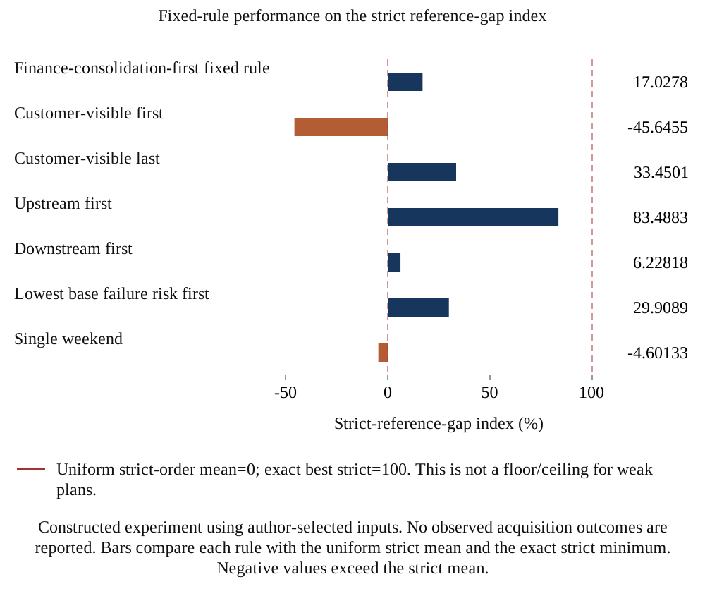
Upstream first follows CM > PC > OM > BI > PA > GL > CS. It ranks 29th and closes 83.49% of the strict reference gap, while remaining 4.73% above the minimum. The fixed finance-consolidation-first order, GL > BI > PA > OM > PC > CM > CS, ranks 1,706th and closes 17.03%. Its order is a benchmark assumption; no measured synergy savings determine it. Customer-visible last closes 33.45%, lowest-base-failure-risk first 29.91% and downstream first 6.23%. Customer-visible first closes minus 45.65%, placing it above the uniform strict mean. The all-seven weekend is also above that mean and is 29.99% above the strict minimum.
Figure 1 presents the reference-gap index with the uniform strict mean at 0 and the strict minimum at 100. Negative bars mean the rule's constructed loss exceeds the reference mean. They do not imply a probability of failure or a negative operational benefit observed at a client. The comparison tests fixed rules against one explicit objective. A buyer can use the same format to expose what a rule omits, then add legal, staffing, service and reversibility constraints before making a live choice. The experiment supplies no evidence that one named rule performs best across businesses.
| Rule | Exact order | Loss (USD thousands) | Gap index | Above strict minimum | Strict rank |
|---|---|---|---|---|---|
| Finance-consolidation-first fixed rule | GL > BI > PA > OM > PC > CM > CS | 371.91 | 17.03% | 23.79% | 1706 |
| Customer-visible first | CS > BI > OM > PA > PC > CM > GL | 425.90 | -45.65% | 41.76% | 4373 |
| Customer-visible last | GL > CM > PC > PA > OM > BI > CS | 357.77 | 33.45% | 19.08% | 931 |
| Upstream first | CM > PC > OM > BI > PA > GL > CS | 314.66 | 83.49% | 4.73% | 29 |
| Downstream first | CS > GL > PA > BI > OM > PC > CM | 381.22 | 6.23% | 26.89% | 2397 |
| Lowest base failure risk first | PC > CM > GL > CS > OM > BI > PA | 360.82 | 29.91% | 20.10% | 1055 |
| Single weekend | one wave | 390.54 | -4.60% | 29.99% | Not a strict order |
Constructed experiment using author-selected inputs. No observed acquisition outcomes are reported. Gap index uses the uniform strict mean as 0 and the exact strict minimum as 100%.
Scroll horizontally to read the figure at full size. You can also open the full-size figure.
Constructed experiment using author-selected inputs. No observed acquisition outcomes are reported. Bars compare each rule with the uniform strict mean and the exact strict minimum. Negative values exceed the strict mean.
A heuristic is useful as a disclosed starting plan and a diagnostic benchmark. Its name is insufficient to reproduce it. A team should record the ordering rule, any tie-break rule and the treatment of systems without inbound dependencies. The comparison here uses the same input set and objective for each plan. A lower loss for an optimised sequence means that the stated objective ranks that sequence above the benchmark. It does not measure the probability that a future acquisition will realise the same saving.
The monetary gap also needs a decision threshold. If two feasible plans differ by less than the uncertainty in the inputs, a buyer can prefer the plan with clearer ownership, a feasible staffing pattern or a more reversible cutover. Those requirements should be recorded as constraints or explicit approval considerations. They should remain visible when the financial ranking is presented. A ranking that silently treats an unavailable implementation team as an executable option creates an operational problem that the numerical loss function cannot resolve.
The finite search and the benchmark comparison answer different questions. Enumeration finds the lowest value of the stated objective within a defined candidate set. A benchmark establishes how a named practical rule compares in that same set. Neither calculation measures the cost of collecting better inputs, changing the integration architecture or negotiating a transition-service extension. Those can be material alternatives before the schedule is fixed. The decision record can therefore place the computed ranking alongside an architecture choice and an information plan, with separate costs and evidence for each.
13 Efficient orders and the placement of systems
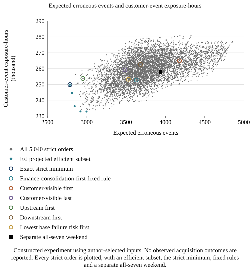
Figure 2 plots every strict order by expected erroneous events E and customer-event exposure-hours J. Its projected efficient subset contains plans for which no other strict order is no worse on both plotted measures and strictly better on at least one. Economic loss also depends on visibility-weighted erroneous events K in equation (3d), so this two-axis projection is not a complete economic frontier. A buyer can inspect these operational outcomes alongside K before accepting the monetary weights. The base-best strict order has 2,785.38 expected erroneous events and 249,838.55 customer-event exposure-hours. The single weekend is shown separately because it belongs to a different family of plans. Its lack of bridge separation does not remove conversion or cutover exposure.
Scroll horizontally to read the figure at full size. You can also open the full-size figure.
Constructed experiment using author-selected inputs. No observed acquisition outcomes are reported. Every strict order is plotted, with an efficient subset, the strict minimum, fixed rules and a separate all-seven weekend.
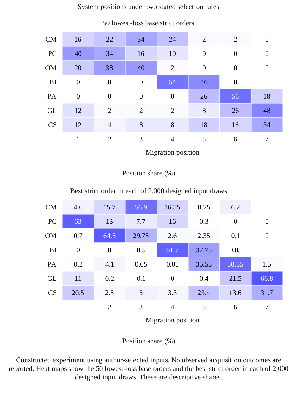
Figure 3 separates two position distributions. The first uses the 50 lowest-loss strict orders at the base inputs; every order has equal weight within that selected set. The second uses the best strict order in each of 2,000 designed input draws; each draw has equal weight. A concentration in a cell describes that particular selection rule and input distribution. It is not a confidence interval for the position a real system should occupy. The base-best sequence puts catalogue and order management ahead of the customer master, illustrating how shorter high-volume interface gaps can outweigh the authored upstream-readiness penalty.
Scroll horizontally to read the figure at full size. You can also open the full-size figure.
Constructed experiment using author-selected inputs. No observed acquisition outcomes are reported. Heat maps show the 50 lowest-loss base orders and the best strict order in each of 2,000 designed input draws. These are descriptive shares.
14 Joint waves and the cost of concurrency
There are 47,293 ordered shared-wave plans across one through seven waves, including the 5,040 strict orders. Enumerating these plans gives a base minimum of USD 275.27 thousand for PC > CM+OM > BI+CS > PA+GL. A plus sign denotes simultaneous migration within one wave. This four-wave minimum is 8.38% below the strict minimum. The best two-wave plan is 1.23% below the strict minimum, while the all-seven single wave is 29.99% above it. The comparison credits shorter interface gaps and exact within-wave exposure union, then charges the assumed concurrency and failure-profile extensions. Feasible staffing and application indivisibility are outside this enumeration.
| Waves | Candidates | Best plan | Loss (USD thousands) | Versus strict minimum |
|---|---|---|---|---|
| 1 | 1 | CM+PC+OM+BI+PA+GL+CS | 390.54 | 29.99% |
| 2 | 126 | CM+PC+OM+GL > BI+PA+CS | 296.73 | -1.23% |
| 3 | 1,806 | GL > CM+PC+OM > BI+PA+CS | 280.10 | -6.77% |
| 4 | 8,400 | PC > CM+OM > BI+CS > PA+GL | 275.27 | -8.38% |
| 5 | 16,800 | PC > CM+OM > BI+CS > PA > GL | 278.44 | -7.32% |
| 6 | 15,120 | PC > OM > CM > BI+CS > PA > GL | 286.91 | -4.50% |
| 7 | 5,040 | PC > OM > CM > BI > PA > GL > CS | 300.44 | 0.00% |
Constructed experiment using author-selected inputs. No observed acquisition outcomes are reported.
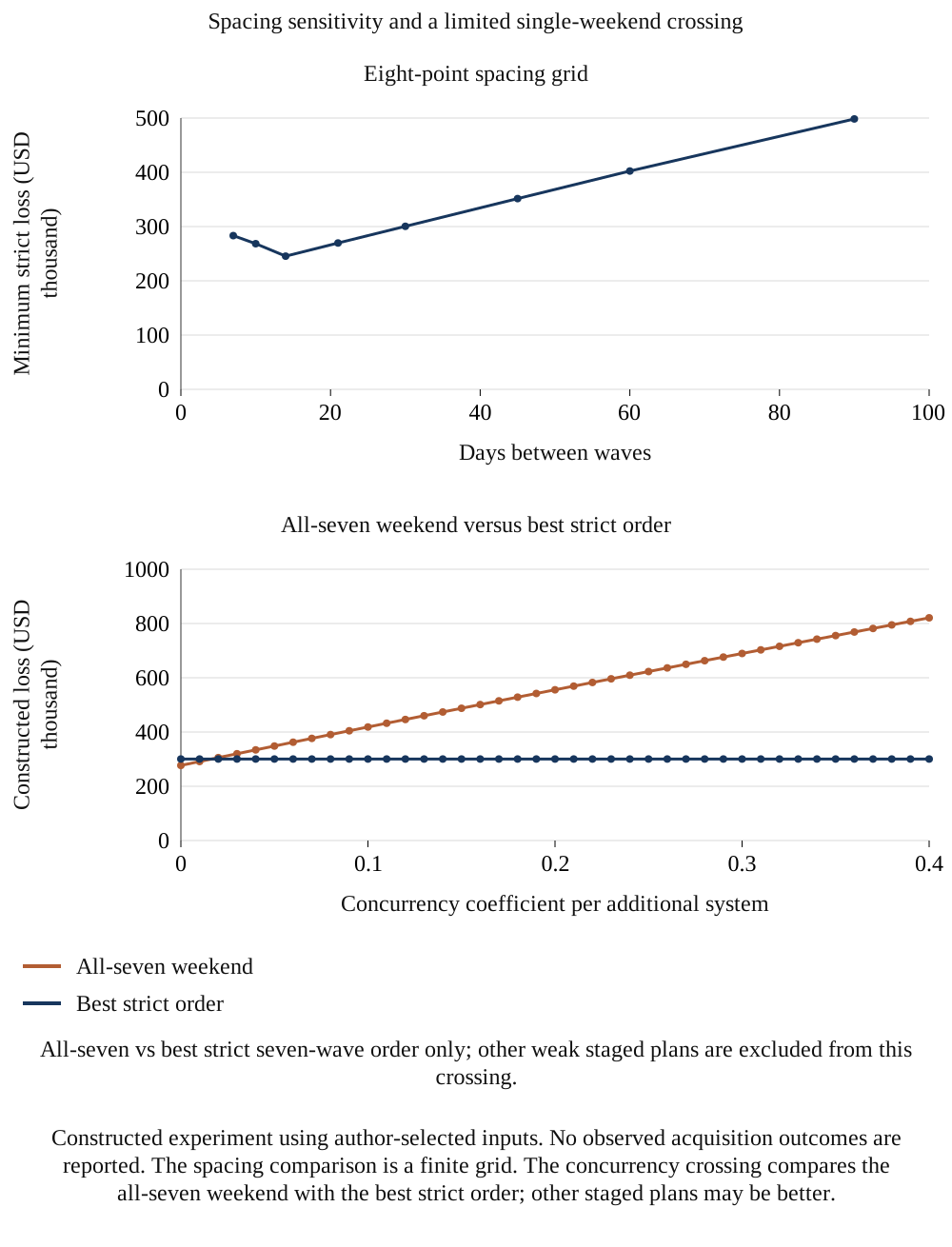
Varying the concurrency coefficient gives a crossing between the all-seven weekend and the best strict order at g_c=0.016385, or about 1.64% per additional concurrent system. This crossing compares those two candidate families only. At that same coefficient, another three-wave plan, GL > CM+PC+OM > BI+PA+CS, has loss USD 258.58 thousand and beats both crossing candidates. A coefficient below the reported crossing therefore does not establish that the single weekend is globally preferred among shared-wave plans. A live joint cutover also requires executable capacity, recovery evidence and legal readiness; an assumed defect coefficient cannot establish those conditions.
Figure 4 also compares eight authored spacing choices: 7, 10, 14, 21, 30, 45, 60 and 90 days, optimising the strict order separately at each choice. The smallest computed loss on this grid is USD 245.44 thousand at 14 days, where the selected order is GL > PC > OM > CM > BI > PA > CS. Fourteen days equals the authored hypercare duration. The kink arises from the specified overlap penalty, and the result is a grid minimum rather than a continuous optimum or an empirical recommendation. The objective excludes the financial value of completing integration sooner and the staffing burden of sustained hypercare. Those omissions require separate evaluation.
Scroll horizontally to read the figure at full size. You can also open the full-size figure.
Constructed experiment using author-selected inputs. No observed acquisition outcomes are reported. The spacing comparison is a finite grid. The concurrency crossing compares the all-seven weekend with the best strict order; other staged plans may be better.
Shared-wave enumeration assumes consecutive wave labels and treats ordering within a simultaneous wave as irrelevant. It does not enumerate hourly task dependencies inside that wave. A coupled application pair may need a release sequence, data freeze, validation step and customer communication before both are treated as available. If those tasks cannot fit within the assumed duration, the four-wave candidate is not yet an executable plan. A detailed runbook can either substantiate the simultaneous-wave approximation or require the candidate to be rebuilt with staggered tasks and different exposure profiles.
15 Stress tests and billing constraints
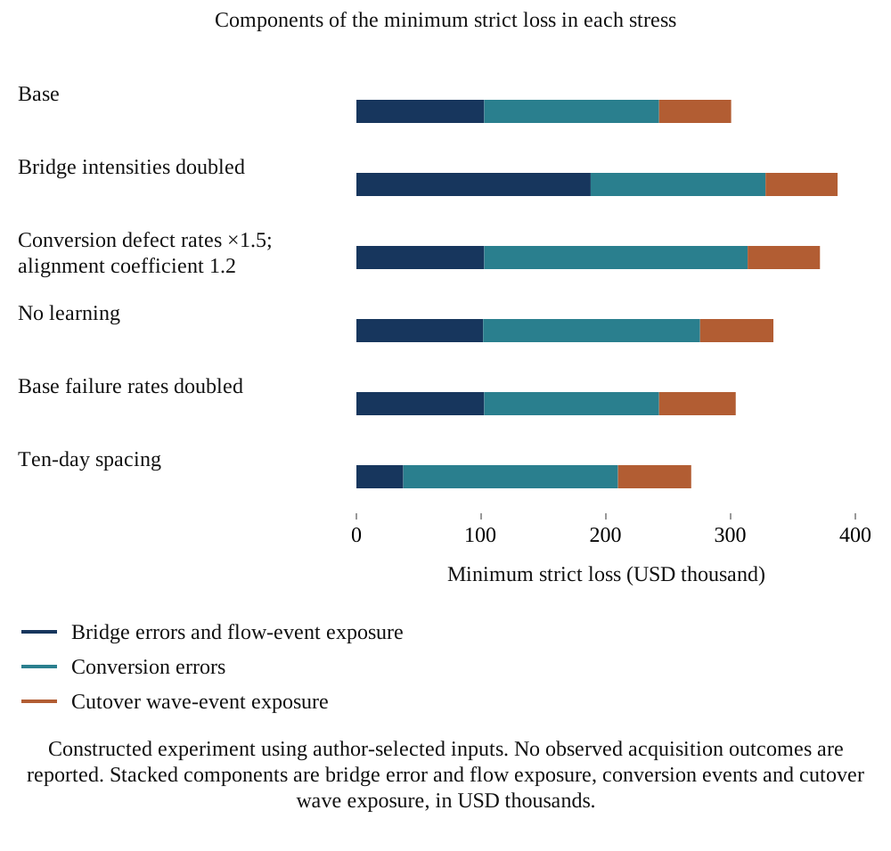
The stress table distinguishes the best plan, the complete ranking and the forecast level. Doubling bridge error intensities preserves the best strict order, but the Spearman correlation of all strict losses is 0.9491 and the complete ranking changes. The new minimum is USD 385.75 thousand, 28.40% above the base minimum. A forecast retaining the original bridge rates would underpredict this stressed level. The scenario changes error intensities and leaves the separate bridge-outage inputs unchanged. That distinction is relevant when identifying which operational measure would need investigation.
Raising conversion defect rates by 50% and doubling the alignment penalty preserves the best order and raises its minimum loss 23.70%, with rank correlation 0.8801. Removing learning changes the final ordering of service and ledger; the base-best order becomes third and has 0.26% regret within that stress. Doubling base failure rates preserves the best order and raises the minimum 1.22%. Its rank correlation is 0.999857, so some orders still reverse. Printing this correlation as 1.000 would conceal those reversals. A stable minimum is a narrower result than an unchanged complete ranking.
With ten-day spacing, the best strict order starts with the ledger and the minimum is USD 268.41 thousand, 10.66% below the base minimum; rank correlation falls to 0.7651. A separate readiness experiment requires planned billing readiness by Day 60 relative to the first cutover at Day 0. Billing requires 24 hours plus an authored two-day acceptance buffer, so at 30-day spacing only its first two wave positions qualify. This leaves 1,440 of 5,040 strict orders feasible. The best feasible sequence is PC > BI > OM > CM > PA > GL > CS, planned ready on Day 33, with loss USD 356.45 thousand, 18.65% above the unconstrained strict minimum. Actual successful readiness and a statutory civil-calendar date are not established by this arithmetic.
| Case | Best order | Loss (USD thousands) | Rank correlation | Base-plan rank | Base-plan regret |
|---|---|---|---|---|---|
| Bridge intensities doubled | PC > OM > CM > BI > PA > GL > CS | 385.75 | 0.949066 | 1 | 0.00% |
| Poor conversion: delta 1.5, kappa 1.2 | PC > OM > CM > BI > PA > GL > CS | 371.63 | 0.880145 | 1 | 0.00% |
| No learning | PC > OM > CM > BI > PA > CS > GL | 334.30 | 0.962511 | 3 | 0.26% |
| Base failure rates doubled | PC > OM > CM > BI > PA > GL > CS | 304.09 | 0.999857 | 1 | 0.00% |
| Ten-day spacing | GL > PC > OM > CM > BI > PA > CS | 268.41 | 0.765069 | 3 | 0.41% |
Constructed experiment using author-selected inputs. No observed acquisition outcomes are reported. All five stresses change the full ranking; retaining the same best order is a narrower result.
Scroll horizontally to read the figure at full size. You can also open the full-size figure.
Constructed experiment using author-selected inputs. No observed acquisition outcomes are reported. Stacked components are bridge error and flow exposure, conversion events and cutover wave exposure, in USD thousands.
Figure 5 decomposes the loss of the best order in each stress. The components help frame questions for a programme review: whether an observed incident belongs to an interface, a conversion or a cutover; whether the plan has changed; and whether the relevant denominator was measured consistently. Similar symptoms can have several causes in an actual business. A rate departure alone does not establish a causal diagnosis or confirm the scheduling choice. Recalculation should follow a review of the event evidence, the assumptions and the constraints rather than a mechanical interpretation of one stress signature.
The relative readiness condition separates three dates: the start of billing cutover, its planned technical finish and the end of the acceptance buffer. A business's civil-calendar plan needs additional items, including the legal effective date, provider accreditation evidence, test exchanges, fallback arrangements and any retained platform that already meets the obligation. A change in the ownership perimeter may alter the scope assessment without moving the technical cutover at all. Treating a statutory date as a fixed wave label would discard those distinctions and could exclude feasible transition arrangements or admit an unready one.
16 Ranking uncertainty across input draws
The input-draw exercise uses 2,000 authored joint draws, with one input vector applied to all 5,040 strict orders within each draw. Independent mean-one lognormal factors have coefficient of variation 0.4 for bridge error rates, conversion defect rates, base failure rates and the alignment penalty; failure-rate inputs are capped at 0.5. Learning coefficient ell is drawn uniformly from 0.02 to 0.12. Durations and erroneous events per defect receive independent mean-one factors with coefficient of variation 0.3. The learning floor remains 0.6. These distributions define the sensitivity experiment. They are not fitted frequencies of migration conditions and are not probabilities about a future client.
The base-best order is best in 364 of 2,000 draws, or 18.2%, with a Monte Carlo standard error of 0.86 percentage points for that frequency. Its mean regret against each draw's strict minimum is 1.48%, with Monte Carlo standard error 0.036 percentage points, and its empirical 95th percentile regret is 4.86%. It lies within 5% of each draw's minimum in 1,912 draws and exceeds 10% regret in two. The most frequent winner is PC > OM > CM > BI > CS > PA > GL, with 419 wins. The order minimising empirical 95th-percentile regret in these same draws is PC > OM > CM > BI > PA > CS > GL, at 4.52%. This is an in-sample choice; there is no independent validation of that quantile criterion.
| Order | Wins /2,000 | Win share | Mean regret | Mean MCSE (pp) | Empirical 95th percentile regret |
|---|---|---|---|---|---|
| PC > OM > CM > BI > CS > PA > GL | 419 | 20.95% | 1.64% | 0.038 | 4.96% |
| PC > OM > CM > BI > PA > GL > CS | 364 | 18.20% | 1.48% | 0.036 | 4.86% |
| PC > OM > CM > BI > PA > CS > GL | 250 | 12.50% | 1.42% | 0.033 | 4.52% |
| CS > CM > OM > PC > BI > PA > GL | 247 | 12.35% | 5.09% | 0.112 | 14.17% |
| CS > PC > OM > CM > BI > PA > GL | 108 | 5.40% | 4.85% | 0.100 | 13.57% |
| CM > PC > OM > BI > PA > GL > CS | 2 | 0.10% | 6.32% | 0.068 | 11.81% |
Constructed experiment using author-selected inputs. No observed acquisition outcomes are reported. Regret uses the draw-specific strict minimum. The p95 choice is selected and evaluated in the same draws.
The upstream-first benchmark has mean regret 6.32% and empirical 95th-percentile regret 11.81% under the chosen draws. These values use loss divided by the draw's minimum, minus 1; they use a different denominator from the strict reference-gap index in Figure 1. Additional deterministic sensitivities vary bridge intensity, alignment, duration, valuation weights and repair cost. One learning sensitivity jointly raises ell from 0.07 to 0.14 and lowers the floor from 0.6 to 0.4. It is a two-input scenario, so its effect cannot be attributed to ell alone. Among these eight scenarios the largest regret of retaining the base-best order is 3.74%, when the alignment penalty is removed. None establishes a general sequencing recommendation.
The uncertainty draws are a designed sensitivity exercise. Their distributions state how the analysis varies authored inputs; they are not estimates of the frequency of real migration conditions. A reader should inspect whether correlations are omitted. A single weak supplier, poor source-data quality or a shared security dependency could raise several rates together. The selection of distributions, dependence structure and stress combinations therefore belongs in the approval record alongside the result. More draws improve the numerical description of the chosen experiment; they do not establish that the chosen experiment represents the business.
For operational use, the team can separate uncertainties that can be reduced before completion from those that remain during execution. Reconciliation samples and rehearsals may inform mapping defects, while a supplier's recovery behaviour may remain uncertain until an incident occurs. The next information-gathering task should target a parameter that could change the choice between feasible plans. Repeatedly refining a parameter that moves every plan's cost by a similar amount can improve the forecast level while leaving the scheduling decision unchanged. That distinction helps direct diligence effort.
| Change | Best strict order | Base-plan regret | Rank correlation |
|---|---|---|---|
| Bridge intensities half | PC > OM > CM > BI > CS > PA > GL | 0.30% | 0.936975 |
| Alignment penalty zero | GL > PA > PC > BI > OM > CM > CS | 3.74% | 0.863066 |
| Alignment penalty doubled | PC > OM > CM > BI > PA > GL > CS | 0.00% | 0.948654 |
| Joint learning change: ell 0.14 and floor 0.4 | PC > OM > CM > BI > PA > GL > CS | 0.00% | 0.989565 |
| Cutover durations doubled | PC > OM > CM > BI > PA > GL > CS | 0.00% | 0.999857 |
| Departure weight per event-hour tripled | PC > OM > CM > BI > CS > PA > GL | 1.62% | 0.991807 |
| Departure weight per visible error tripled | PC > OM > CM > BI > PA > GL > CS | 0.00% | 0.998954 |
| Error repair cost doubled | PC > OM > CM > BI > PA > GL > CS | 0.00% | 0.999478 |
Constructed experiment using author-selected inputs. No observed acquisition outcomes are reported. The learning row changes two inputs together; all other listed rows change the stated input family.
17 Outcome variation across simulated programmes
A separate experiment generates 5,000 programme outcomes for each of seven strict-order choices. Flow-specific and system-specific mean-one gamma factors with coefficient of variation 0.35 vary error intensities, and Poisson draws generate event counts. Cutover failures use the specified system probabilities. Bridge-outage exposure uses its conditional mean multiplied by the flow factor; it does not simulate individual outage timestamps or a customer-level outage process. The base-best plan's simulated mean is USD 299.50 thousand with Monte Carlo standard error USD 410.48, compared with analytic expectation USD 300.44 thousand. Its empirical 5th-to 95th-percentile interval is USD 255.25 thousand to USD 351.07 thousand.
| Plan | Mean (USD thousands) | Mean MCSE (USD) | 5th percentile (USD thousands) | 95th percentile (USD thousands) |
|---|---|---|---|---|
| Best strict | 299.50 | 410.48 | 255.25 | 351.07 |
| Finance-consolidation-first fixed rule | 370.59 | 647.81 | 301.47 | 450.01 |
| Customer-visible first | 424.60 | 689.94 | 349.97 | 509.47 |
| Customer-visible last | 356.81 | 450.95 | 306.81 | 411.64 |
| Upstream first | 313.61 | 429.05 | 266.71 | 366.09 |
| Downstream first | 379.86 | 608.07 | 313.94 | 454.52 |
| Lowest base failure risk first | 359.92 | 473.31 | 306.31 | 416.27 |
Constructed experiment using author-selected inputs. No observed acquisition outcomes are reported. 5,000 outcomes per plan; flow/system gamma heterogeneity, Poisson errors and system failure draws.
Two comparison designs are reported separately. Shared conditions reuse complete uniform and gamma draws for both plans, producing a paired numerical comparison. Separate-programme comparisons generate an independent set of draws using a second seed. Against upstream first, the base-best order has lower loss in 97.06% of paired draws and 64.38% of independent-programme pairings; the latter frequency has Monte Carlo standard error 0.68 percentage points. Independent comparisons are illustrations of variability under this authored process, not an observational study of different acquisitions. Even a frequency of 100% in 5,000 draws does not establish a probability of 1 or a guaranteed result.
The Monte Carlo standard error describes numerical uncertainty in a reported mean or frequency under the specified generator. It does not include uncertainty about the generator's suitability. A zero estimated standard error for a win frequency observed in every simulated pairing is a property of that plug-in calculation, and carries no guarantee about a new draw. Reporting the draw count and comparison design keeps the result interpretable. The independent sample comparison also does not reproduce the common economic, supplier or regulatory shocks that several actual deals might share; those require a separate dependence specification.
| Benchmark | Paired lower-loss share | Paired MCSE (pp) | Independent lower-loss share | Independent MCSE (pp) |
|---|---|---|---|---|
| Finance-consolidation-first fixed rule | 100.00% | 0.000 | 91.68% | 0.391 |
| Customer-visible first | 100.00% | 0.000 | 99.18% | 0.128 |
| Customer-visible last | 100.00% | 0.000 | 91.20% | 0.401 |
| Upstream first | 97.06% | 0.239 | 64.38% | 0.677 |
| Downstream first | 100.00% | 0.000 | 94.88% | 0.312 |
| Lowest base failure risk first | 100.00% | 0.000 | 91.86% | 0.387 |
Constructed experiment using author-selected inputs. No observed acquisition outcomes are reported. Each share compares the base-best strict order with the benchmark across 5,000 paired or independently generated samples. An observed 100% is not a guarantee.
18 Calibration using constructed programme logs
A firm estimating rates from its history would divide interface-error counts by separated-platform transaction exposure, and attributed conversion-error events by the full event exposure N_s x_s M_sm. These ratios of totals can be computed from a programme log and audited against the recorded denominators. With known exposures and stable rates, repeated use of any fixed strict order in this network supplies positive bridge and conversion denominators and can identify those rates. A fixed order does not, by itself, separately identify a learning curve from unrestricted system-specific rates. Variation in positions supplies additional identification evidence, while judgement-based scheduling can confound structural effects with the reasons for that judgement.
Here m indexes constructed logged programmes, C^B counts interface errors and C^C counts erroneous events attributed to conversion. The full conversion multiplier M_sm includes alignment, learning, concurrency and overlap. Omitting its last two factors would give an incomplete exposure denominator when waves are shared or hypercare overlaps. The experiment uses independently randomised full strict orders and assumes the complete structure and all non-rate inputs are known. Gamma rate factors with coefficient of variation 0.7 introduce between-programme heterogeneity. Rate estimates are inserted into the objective, a strict order is selected and its loss is evaluated using the original true inputs. Each sample size has 300 replications.
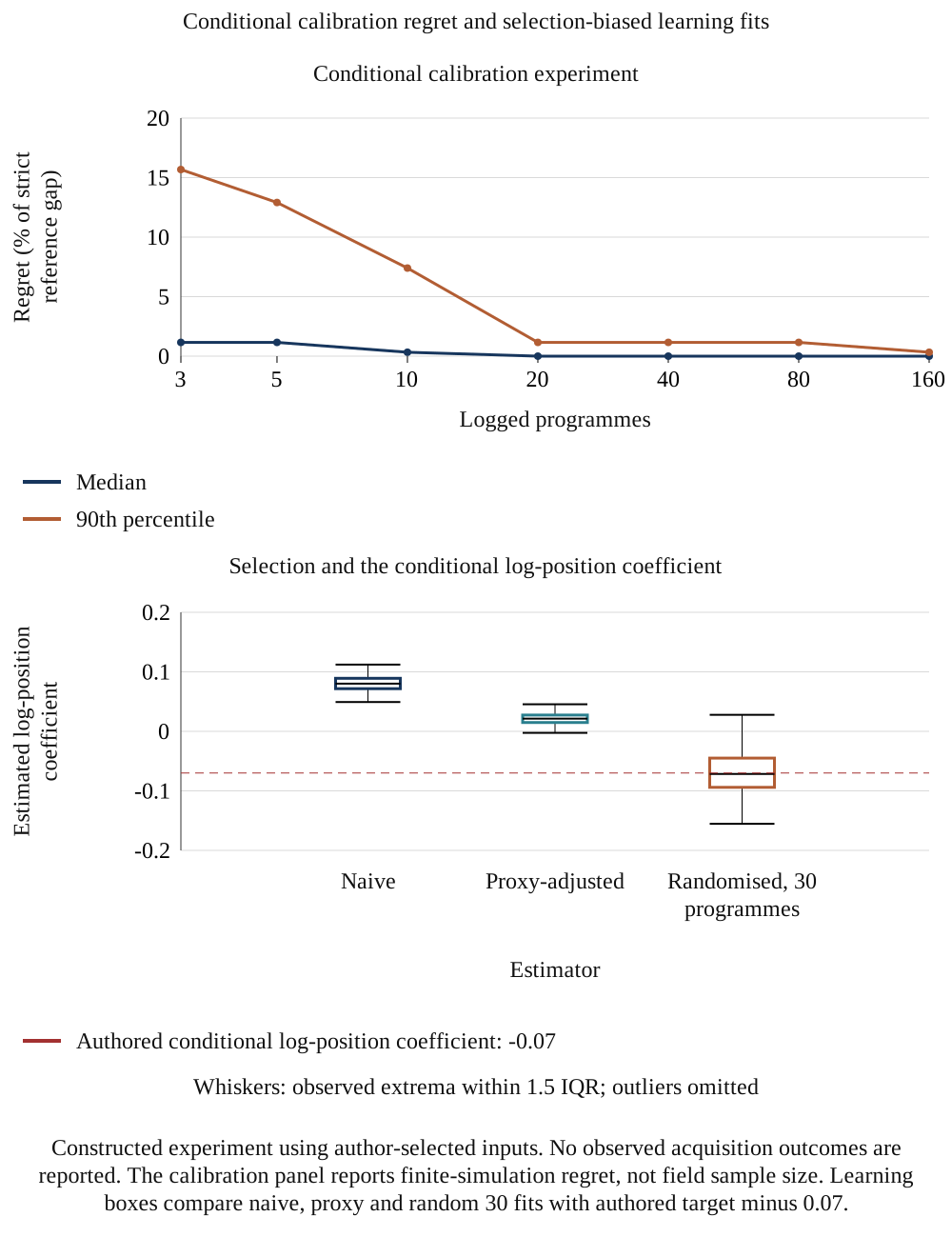
At three programmes the median selected-order regret is 1.16% of the strict reference gap and the 90th percentile is 15.68%. At ten programmes they are 0.33% and 7.40%, and all 300 selected orders lie in the base top 50. Ten is the first tested grid value whose empirical 90th-percentile gap regret is at most 10%. This is a conditional result for the simulated design. It is not a sufficient sample size, a formal lower bound on field requirements or evidence of finite-sample unbiasedness. At 40 programmes the mean estimated-to-true bridge-rate ratio is about 1.0046; this numerical mean does not establish an estimator property. Actual requirements depend on incident rates, exposure variation, missingness, dependence and the precision needed for a live decision.
| Programmes | Replications | Median gap regret | p90 gap regret | Top-50 count /300 | Mean-regret MCSE (pp) |
|---|---|---|---|---|---|
| 3 | 300 | 1.16% | 15.68% | 289 | 0.425 |
| 5 | 300 | 1.16% | 12.91% | 295 | 0.377 |
| 10 | 300 | 0.33% | 7.40% | 300 | 0.221 |
| 20 | 300 | 0.00% | 1.16% | 300 | 0.117 |
| 40 | 300 | 0.00% | 1.16% | 300 | 0.027 |
| 80 | 300 | 0.00% | 1.16% | 300 | 0.023 |
| 160 | 300 | 0.00% | 0.33% | 300 | 0.018 |
Constructed experiment using author-selected inputs. No observed acquisition outcomes are reported. Known structure, randomly assigned full orders and gamma rate heterogeneity CV 0.7. No field sufficiency or power claim.
Zero exposure requires an explicit treatment in a field estimator. If two systems always move together, their interface has no separated-platform exposure in those programmes, so the corresponding bridge rate cannot be estimated from a zero denominator. A positive numerator paired with zero measured exposure indicates a definition or recording problem to investigate. Conversion estimates likewise depend on attributing erroneous events to converted records and recording the applicable multipliers. These requirements can make the usable sample smaller than the number of completed deals. A log-quality assessment should precede any claim that a retained history supports calibration.
19 Selection bias in estimated learning
The selection experiment assumes that teams observe a noisy signal of a programme-system's latent fragility and place apparently fragile systems later. This is an authored scheduling mechanism, not a claim about how all acquisition teams behave. Each replication generates 120 selected programmes and a separate collection of 120 fully randomised strict-order programmes. Latent fragility has normal standard deviation 0.5; perception noise also has standard deviation 0.5. Conversion defect counts follow a conditional Poisson mean with the same base exponential learning curve. At these seven positions the floor is inactive, so the true log-position coefficient is minus 0.07.
D_ms denotes converted-record defects for system s in programme m, rather than downstream erroneous transaction events. The latter additionally multiply by x_s in the loss model. W_m is the full seven-system wave-position vector; it determines U_ms as well as the system's own position w_ms. Eta_ms is latent fragility and the normalisation minus sigma_eta squared over 2 gives its exponential factor mean 1. Selected programmes use ascending rank of fragility plus perception noise. The fitted working log mean is log(N_s delta_s U_ms) + alpha + b(w_ms - 1), where alpha is an estimated intercept; the proxy-adjusted fit also adds gamma z_ms. The rating z_ms equals latent fragility plus independent normal noise with standard deviation 0.5. The randomised comparisons fit either the first 30 or all 120 programmes from the separately randomised collection. No partial within-programme randomisation is simulated.
| Estimator | Programmes | Mean coefficient | Coefficient MCSE | Coefficient SD | Mean gap regret | p90 gap regret |
|---|---|---|---|---|---|---|
| Selected orders; naive fit | 120 | +0.08059 | 0.00093 | 0.01320 | 1.16% | 1.16% |
| Selected orders; noisy proxy | 120 | +0.02178 | 0.00077 | 0.01094 | 0.51% | 1.16% |
| Randomised full orders; 30 programmes | 30 | -0.07051 | 0.00235 | 0.03320 | 0.18% | 0.33% |
| Randomised full orders; 120 programmes | 120 | -0.07058 | 0.00119 | 0.01689 | 0.05% | 0.33% |
Constructed experiment using author-selected inputs. No observed acquisition outcomes are reported. 200 replications; target log-position coefficient minus 0.07. random30 and random120 use a separately generated randomised collection.
Across 200 replications the naive mean log-position coefficient is plus 0.08059 with Monte Carlo standard error 0.00093, and the proxy-adjusted mean is plus 0.02178 with standard error 0.00077. Both have the opposite sign to the authored minus 0.07. The 30-programme randomised fit averages minus 0.07051 with standard error 0.00235; using all 120 gives minus 0.07058 with standard error 0.00119. Means close to the target do not prove unbiasedness. After fitting, the floored exponential curve is passed into the full plan calculation. Mean selected-order gap regret is 1.16% for the naive fit, 0.51% for the proxy fit, 0.18% for random 30 and 0.054% for random 120. Ignoring learning produces 0.33% gap regret in this case.
Scroll horizontally to read the figure at full size. You can also open the full-size figure.
Constructed experiment using author-selected inputs. No observed acquisition outcomes are reported. The calibration panel reports finite-simulation regret, not field sample size. Learning boxes compare naive, proxy and random 30 fits with authored target minus 0.07.
The conditional generator in equation (5a) has an exact exponential mean while the floor is inactive. The working naive and proxy regressions use known exposure offsets and do not observe latent fragility; the proxy supplies only a noisy measure. Under selected scheduling, their fitted conditional means need not equal the generator's conditional mean. Actual rates and readiness measures would themselves be estimated and can correlate with scheduling decisions. A proxy can reduce one source of confounding while leaving others. In a field study, the assignment unit, eligibility rules, exclusions and clustering would need to be set before interpreting a coefficient as a learning effect. Comparing a model-selected order with an observed outcome also requires a protocol for changes made after scheduling and for incidents discovered outside the measurement window.
20 Numerical verification and structural limits
The constructed outcomes use the same operational relationships that define the decision model. This makes the experiment useful for checking the method's arithmetic, its response to assumptions and the consequences of estimation error. It supplies no independent empirical test of those relationships. A favourable comparison with a simple ordering rule establishes a result within the constructed setting. Validation against acquisition outcomes would require recorded exposures, consistently defined error events and a design that addresses how teams select their migration plans.
Nineteen numerical control groups pass. Independent scalar reconstructions of every strict order agree with the vectorised loss under both the base learning curve and a custom curve, with maximum absolute residual below USD 0.000000001. Exact within-wave integrals match an independent inclusion-exclusion calculation across all 127 non-empty system subsets. Component totals reconcile across all 52,333 candidate rows evaluated in the strict and shared-wave collections, with the strict collection also present inside the shared-wave set. Further checks cover input rejection, failure bounds, zero-inbound systems, the inactive base learning floor, full calibration denominators, position marginals and input-draw frequencies. These tests check implementation consistency; they do not validate authored rates or structural assumptions against real acquisitions.
| Control group | Result and scope |
|---|---|
| within wave integral 127 subsets | Pass; max_hours_residual=1.4210854715202004e-14 |
| scalar all 5040 default | Pass; max_USD_residual=1.7462298274040222e-10 |
| scalar all 5040 custom learning | Pass; max_USD_residual=1.7462298274040222e-10 |
| counts | Pass; strict=5040, weak=47293 |
| component identity all 52333 | Pass |
| strict proxy identity | Pass |
| source zero inbound | Pass |
| floor inactive base | Pass; last_factor=0.6570468198150567 |
| failure bounds | Pass |
| no bridges single | Pass |
| calibration full multiplier base | Pass |
| calibration full multiplier ties | Pass |
| calibration full multiplier overlap | Pass |
| invalid share duration rejections | Pass; cases=6 |
| invalid scalar custom curve rejections | Pass; cases=3 |
| position marginals | Pass |
| draw best frequencies | Pass |
| same curve in selection | Pass |
| immutable snapshot hashes | Pass; files=13 |
Constructed experiment using author-selected inputs. No observed acquisition outcomes are reported. 19 groups; implementation consistency only, without empirical structural validation.
Reproduction uses fixed seeds and separate stored outputs for distinct exercises: input draws, shared-condition outcomes, independently generated outcome samples, rate calibration and selection-biased learning. The six figures are projections of those stored values. Quantiles use linear interpolation over the stated samples. The empirical 95th-percentile choice is evaluated on the same input draws used to select it, so it carries selection optimism that the present exercise does not estimate. Repeating a seed can verify a computation; evidence from another measured population would be needed to examine transportability.
| Exercise | Seed | Finite sample | Generation and comparison scope |
|---|---|---|---|
| Joint input draws | 777 | 2,000 vectors, each shared by all 5,040 strict orders | Independent mean-one lognormal factors: CV 0.4 for bridge rates, defect rates, base failure probabilities and alignment penalty; CV 0.3 for durations and events per defect. Drawn base failure probabilities are capped at 0.5; learning ell is uniform from 0.02 to 0.12. Other inputs remain fixed. |
| Programme outcomes | 31415 and 99 | 5,000 outcomes per strict plan in each collection | Independent mean-one gamma flow/system factors with CV 0.35, Poisson error counts and system failure draws. Bridge exposure uses the same flow factor. Shared-condition comparisons reuse the complete 31415 collection; independent comparisons pair the best plan's 31415 outcomes with the benchmark's separately generated 99 outcomes. |
| Rate calibration | 2718 | 300 replications for each programme count 3, 5, 10, 20, 40, 80 and 160 | Independent random full strict orders and mean-one gamma rate heterogeneity with CV 0.7; Poisson error counts, known full exposures and known non-rate inputs. The selected order is evaluated at the true base inputs. |
| Learning selection | 4242 | 200 replications; 120 selected and a separate 120 randomised programmes per replication | Independent zero-mean normal latent fragility, perception noise and proxy noise, each with standard deviation 0.5; conditional Poisson defect counts. Random 30 uses the first 30 programmes of the randomised 120 collection. Fits use the stated known offset, intercept and optional noisy proxy; the base learning floor is inactive. |
All distributions are authored. Quantiles use NumPy linear interpolation. Mean MCSE uses sample standard deviation with one degree of freedom correction divided by the square root of the replication count; share MCSE uses the plug-in binomial formula. A zero boundary estimate does not establish certainty. The empirical p95 plan is selected and evaluated on the same input draws, without held-out validation.
21 Design of a study using migration logs
No acquisition-level client logs are used in this study. Its evidence consists of the documented public sources and a constructed experiment. A proposed field study would define its unit as a cutover wave within a programme and record planned and actual cutover times, the systems moved, the flows bridged and the errors detected. It would use an agreed classification that allows bridge, conversion, other and unresolved causes, define outcomes before collection and pre-register the analysis plan, including the estimators in equations (4a) and (4b). Programme and firm clustering, eligibility and lawful data access would need explicit treatment.
The proposed register would include abandoned, paused and rolled-back programmes as well as completed programmes, so the sampling frame and missing outcomes remain visible. A randomised slice would be limited to operationally eligible alternatives approved before assignment, with explicit allocation, adherence, interference and safety rules. Its causal interpretation would depend on those conditions and the analysis, rather than follow automatically from randomisation. Customer and employee information would require a documented lawful basis or authority, appropriate permissions and safeguards. Aggregating counts does not by itself establish that people cannot be identified, particularly when cells are small or linked with other information. The study would assess identifiability, minimise access and agree retention and sharing controls before collection. [17]
A useful study size cannot be inferred from the constructed calibration exercise alone. It depends on variation in migration plans, incident rates, differences between businesses and the precision required for the decision. An initial research stage should estimate those quantities, specify a practically material loss or exposure difference and calculate a design-specific sample requirement. Programme-level clustering matters because several waves in one acquisition share a team, architecture and management process. Rehearsal records can help test data definitions and instrumentation before a firm seeks to combine evidence across acquisitions.
| Element | Specification | Reason |
|---|---|---|
| Unit | One cutover wave in one programme, with systems moved and flows bridged | Order and exposure are defined at wave level |
| Timestamps | Planned and actual cutover, bridge start and end, first and last error, hypercare close | Days apart and the clock on every outcome |
| Outcomes | Erroneous events by class; additive customer-event exposure-hours; separately defined actual customer and cash outcomes | Keep constructed estimands distinct from measured field outcomes |
| Inclusion | All programmes started, including abandoned and rolled-back | Avoid selection on completion |
| Randomised slice | Pre-approved eligible alternatives; allocation and clustering recorded; adherence, interference and safety monitored | Estimate the pre-specified contrast subject to assignment, adherence, measurement and analysis conditions |
| Lawful authority, permissions and data protection | Applicable regime and lawful basis or authority; minimised data; identifiability assessment; consent where required; controlled retention and sharing | Limit collection and re-identification risk; document the applicable duties and safeguards |
| Analysis plan | Registered estimators with programme-level variation; predicted against observed loss | Limit analytic freedom |
Proposed study design. Entries describe what to collect and why; no such study has been run.
The UAE federal Personal Data Protection Law defines personal data to include indirect identification through linkage. Its territorial scope and exclusions require attention to government, separately regulated health and banking or credit data and free-zone entities with their own data-protection legislation. Article 4 specifies cases permitting processing without the data subject's consent, subject to the applicable conditions; Articles 5 and 6 address processing controls and consent where used. [17] A proposed study would identify the applicable federal, DIFC, ADGM or other special regime before access or sharing, and separately address cross-border transfers where relevant. This limited statutory context does not establish that a particular log, aggregate, consent process or research project is compliant.
22 Board reporting and approval evidence
The board report should disclose the sequence, feasible alternatives and the evidence available when the choice was made. It should link each wave to an interface register, an accountable operating owner, a tolerance, recovery evidence and any external date. Forecasts should distinguish transaction-error events, customer-event exposure-hours, repair expenditure and the annual-revenue-equivalent index. Each input should have a recorded basis: author-selected for an exploratory comparison, measured in a rehearsal or estimated from a defined programme population. The report should identify which items remain provisional and what decision depends on resolving them.
The 5th-to 95th-percentile interval from the constructed outcome simulation spans about USD 95.81 thousand, compared with the strict reference gap of USD 86.15 thousand. That comparison illustrates variation within the stated stochastic model. It is not a prediction interval calibrated for the acquisition under approval. A board needs the uncertainty that relates to its own choices: whether a plan is executable, whether a customer obligation can be met and whether evidence supports its financial exposure assumptions. Realised outcomes can prompt investigation, while an evaluation of the original decision also requires the information and options available at the time.
| Item | Content | Why the board needs it |
|---|---|---|
| Wave plan | Systems per wave, order and the reason for each position | Shows the decision and the coupling it respects |
| Bridge register | Flows bridged, volume, error rate and days bridged | Shows measured or estimated interface exposure under the stated perimeter |
| Tolerances and rollback | Maximum tolerable downtime, cutover window and last rollback point per wave | Shows what failure would mean |
| Compliance calendar | Dates, provider appointment and which wave billing must join | Shows external constraints on the order |
| Forecast range | Error events, customer-event exposure-hours, repair cost and annual-revenue-equivalent index, with input provenance | Separates the conditional calculation from measured outcomes and cash effects |
| Gate evidence | Rehearsal results, open defects and hypercare error counts before each wave | Authorises the next wave |
Proposed reporting. Entries describe the content of the report; they are not findings about a particular programme.
Approval evidence should remain linked to the version of the plan it supports. If a supplier changes a release, the team moves a wave or the legal perimeter changes, the earlier rehearsal may no longer test the proposed configuration. The report should identify the affected assumptions and the tests that need to be repeated. A controlled revision history allows the board to see what management knew when it approved a decision. It also supports later analysis of whether an unexpected outcome arose from a changed plan, an incorrect input or a limitation of the model.
The loss comparison should be reconciled to the deal's value-creation plan before any benefit is booked in management reporting. The objective already includes error-correction cost and revenue-weighted exposure. Adding its full reduction to separate remediation and retention savings could count the same effect twice. A synergy tracker should identify the baseline, the causal mechanism, the period, the accountable owner and any overlap with other benefits. Cash release from a receivable timing change should be reported separately from recurring operating savings and from an assumed reduction in annual revenue exposure.
23 Preparing Day One and the interim operating model
Day One requires continuity of the services and controls needed to operate the acquired business. Full platform consolidation can follow a different timetable. The buyer should identify which customer, billing, payment and reporting processes must function immediately after completion and which can remain supported by an interim arrangement. That distinction is a design input to the migration problem. A legally completed acquisition does not by itself identify the systems the buyer controls, the rights it has to use a supplier's platform or the evidence needed to change an interface.
The acquisition agreement and transition-service arrangements need to be reflected in the plan. A retained seller service may have a termination date, a defined support level and a charge for extending it. Those features can constrain the last feasible migration wave and the available recovery route. The constructed objective does not price contractual transition services. In a transaction, finance and legal teams should identify those costs and constraints before comparing alternatives. An extension that preserves a tested recovery route can have a different economic effect from an extension that merely postpones unresolved mapping work.
The timeline below is a proposed control sequence. It uses decision events rather than prescribing a universal number of days after closing. Each transaction should supply its own dates, governing obligations and acceptance evidence. A programme that has not established a workable interim process should expose that gap before completion. The appropriate response can involve changing the transaction timetable, extending a service arrangement or retaining a system temporarily. Those choices require transaction-specific approval and cannot be inferred from the seven-system numerical example.
| Decision event | Evidence required | Approval question |
|---|---|---|
| Before signing | Systems perimeter, critical processes and seller dependencies | Can the proposed transaction operate through the interim state? |
| Before completion | Access rights, tested interfaces, reconciliation and recovery routes | Which services can transfer with the required support? |
| Day One | Named operating owners, exception queues and opening control evidence | Are critical transactions being processed and reconciled? |
| Before each later wave | Current rehearsal, defect disposition, calendar and recovery evidence | Does this configuration meet its agreed acceptance conditions? |
| After the final wave | Residual transactions, access review and interface retirement record | Which interim services can be closed without leaving obligations unsupported? |
Authored implementation framework. The events require transaction-specific dates and approvals; no observed implementation outcome is claimed.
Opening balances and unresolved transactions deserve explicit ownership. An invoice created before completion may be collected after the ledger or customer master has moved. Credit notes, disputes and unapplied receipts can cross the same boundary. The plan should identify the record of authority, the route for a correction and the reconciliation that connects old and new identifiers. These items can remain financially material after the headline cutover has succeeded. Their treatment should be tested with representative cases before the relevant interface or seller service is retired.
A change in the legal or tax perimeter can also change what a technically valid transaction means. The payer, invoice issuer, service provider and contracting customer may be different legal persons. Entity identifiers should therefore be part of the mapping and acceptance record. The graph in the numerical case describes software functions and data flows. Applying it to a transaction requires a separate mapping to the entities and obligations that those functions serve. The chosen order should be reconsidered when that mapping changes.
24 Assigning responsibility and testing automated mappings
A sequence becomes executable when each decision has an accountable owner, a person responsible for the work and a stated source of acceptance evidence. A single programme manager can coordinate the schedule while operational owners remain responsible for the services they run. Finance should participate in decisions that affect billing, cash application, the ledger and the reporting of benefits. Legal and data-protection specialists should review the obligations within their remit. The role names below are proposed responsibilities; each buyer should assign actual people and resolve gaps before a wave starts.
| Decision | Accountable role | Responsible role | Acceptance evidence |
|---|---|---|---|
| Customer and entity identity | Commercial operations owner | Data migration lead | Approved matching rules and unresolved identity exceptions |
| Prices, orders and invoices | Order-to-cash process owner | Application and reconciliation leads | Reconciled representative transaction paths |
| Receipts and ledger posting | Finance control owner | Treasury and accounting leads | Cash application and posting reconciliation |
| Cutover and recovery | Service owner | Technical cutover lead | Rehearsal, recovery boundary and incident ownership |
| Regulatory calendar | Relevant compliance owner | Legal, tax and operational specialists | Applicable entity obligations and accepted dates |
| Wave approval | Authorised programme sponsor | Programme manager | Current evidence pack and explicit exceptions |
Authored role framework. Accountable means ownership of the decision; responsible means performance of the work. Consultation and approval rights depend on the transaction's governance.
Automation can support the preparation of those records. Deterministic tests can compare counts, control totals, identifier uniqueness, field formats and the disposition of every rejected record. A semantic matching tool can propose possible links between customer or product records, but a proposed link needs evidence before it becomes an operating instruction. Similar names, reused codes, changed addresses and incomplete tax identifiers can create ambiguity. The acceptance process should identify which mappings can be approved automatically under a tested rule and which require a named reviewer.
Any use of machine learning to suggest mappings is a proposed implementation aid outside the numerical experiment. The paper estimates no accuracy or productivity benefit for such a tool. The buyer should retain the input version, proposed match, supporting fields, confidence information where meaningful, reviewer decision and downstream test result. A change to the tool or its rules should trigger a defined retest. The sequencing model should receive accepted dependencies and measured error information. It should not treat an unreviewed model suggestion as an established relationship between systems.
Reconciliation should test complete transaction paths as well as individual fields. A correctly formatted customer identifier can still point to the wrong legal person. An accepted invoice message can still fail in cash application or be posted to the wrong ledger account. Representative tests should therefore connect the order, invoice, payment, posting and service response, with exceptions retained for investigation. Passing a schema test establishes conformity to that schema. Operational acceptance requires evidence relevant to the transaction's financial and customer consequences.
Exception ownership matters when the same event appears in more than one queue. A service case, failed payment application and ledger adjustment can describe different consequences of one mapping defect. The incident record should connect those observations without discarding the separate work they create. That record supports both operational recovery and the study's event definitions. Without a consistent attribution rule, observed error counts can change when the organisation changes its queue structure, even if the underlying migration quality is unchanged.
25 Tracking financial effects without counting benefits twice
The proposed synergy tracker separates the mechanism of a financial effect from the date on which management reports it. Interface retirement may reduce a recurring service charge. A smaller error queue may reduce remediation effort. Faster collection may change receivable timing. Customer retention may affect future contribution. Those effects have different measurement bases and can overlap with the loss function's components. The tracker should state the counterfactual and the evidence needed to distinguish a migration effect from a change in volume, pricing, staffing or market conditions.
| Effect | Measurement basis | Evidence | Overlap check |
|---|---|---|---|
| Interface or transition-service cost | Contract cost over an identified period | Contract, termination condition and actual invoices | Other service-retirement benefits |
| Remediation effort | Error events and cost to resolve them | Consistent incident records and resource data | Error-correction term already in the objective |
| Receivable timing | Collection dates and outstanding balances | Matched invoice, receipt and cash-application records | Recurring earnings and revenue exposure |
| Customer retention | Defined customer cohort and contribution horizon | Renewal, churn and reason-code evidence | Revenue-weighted exposure and commercial initiatives |
| Recurring operating benefit | Measured cost or contribution against a stated baseline | Comparable operating and financial records | Benefits claimed by adjacent integration workstreams |
Management-analysis framework; accounting treatment and valuation require transaction-specific assessment. Entries are categories of evidence, not realised savings.
A forecast reduction in exposure should retain its forecast status until the evidence changes. Management can record the selected plan and its expected consequences at approval, then compare realised events with the forecast range. An apparent improvement should be investigated for changes in transaction volume, customer mix and detection practice. A favourable outcome from one programme cannot isolate the contribution of its migration order. Recording that distinction allows the financial case to evolve as evidence accumulates without converting the constructed example into a claim about delivered value.
The finance team should also distinguish a commitment from an avoidable cost. A supplier charge may continue until a contractual exit condition is met, even when technical use has stopped. Conversely, keeping a recovery option available may create an explicit temporary expense. The timing of that expense belongs in the transaction's cash plan. The model's operational ranking should be reconciled with such commitments before management treats a lower computed loss as a fundable reduction in acquisition costs.
This reporting discipline gives the sponsor a practical way to commission additional work. If interface exposure dominates, the next task can be a review of mapping and reconciliation. If cutover recovery dominates, the next task can be a tested recovery design and supplier response plan. If legal dates determine feasibility, the next task can be an entity-specific compliance calendar and an accepted interim process. The numerical comparison identifies the assumptions that matter within the model. The evidence register identifies which of those assumptions management can substantiate and which require further investigation.
26 Applying the framework to a transaction
A proposed application begins by defining the decision perimeter: applications, data functions, legal entities, regions, suppliers and transition services. Functions that cannot be migrated separately should be grouped before plans are enumerated. The team then maps directed interfaces with compatible transaction denominators, identifies the applicable invoice and reporting obligations and builds a dated civil-calendar plan. A legal obligation belongs to its actual entity and transaction scope. The relative Day 60 example supplies a method for imposing a planning condition, and supplies no legal conclusion about that acquisition.
The next step is to build a feasible candidate set. Coupled systems can be compared in adjacent or shared waves, subject to staffing, rehearsal, access and recoverability constraints. Fixed ordering rules provide transparent benchmarks, and the loss objective exposes their trade-offs under the selected inputs. Management should then test the parameters most capable of changing the choice. The base case here favours a four-wave plan and places upstream first near the best strict order; another network may favour different groupings or retained coexistence. The documented rationale should cover those alternatives before sequence approval.
During execution, the wave gate should refer to the configuration actually tested. Changes to a vendor release, interface, control owner or cutover date need a documented assessment of affected assumptions and evidence. Incident logs should retain denominator, timing, attribution uncertainty and resolution status, including paused or reversed work. Updated calculations can support a revised decision after the evidence review. Completion reporting should reconcile service continuity, open transactions, retired interfaces and financial effects. It should preserve the difference between a modelled exposure reduction, a reconciled accounting amount and collected cash.
27 Limitations and further research
All operating rates, valuation weights and stochastic input distributions in the experiment are authored. Public evidence comes from selected UK and U.S. failure cases, integration research, U.S. continuity guidance and UAE and Saudi invoice obligations. These sources motivate mechanisms and planning questions; none makes the constructed distributor representative of those jurisdictions or of global mid-market acquisitions. The graph has seven systems and excludes staffing limits, vendor lead times, security architecture, licence conditions and several legal and contractual constraints. Different perimeters can change both the feasible set and its ranking.
The model adds customer-event exposures across waves and interfaces and applies a linear revenue-equivalent weight. It does not deduplicate customer-clock hours across the whole programme or estimate customer departure behaviour. Exposure membership is independent within a wave, starts are simultaneous and failure repeats the whole profile. The joint input-draw exercise also assumes independent factors where a common supplier or data-quality weakness could create dependence. Learning, overlap and concurrency are simple functional forms. The single-weekend crossing concerns the best strict order and excludes better shared-wave alternatives. Each limitation narrows the interpretation of the reported numerical results.
Further research could compare alternative exposure dependence models, resource-constrained calendars, variable-duration hypercare and customer-specific recovery timelines. It could test whether interface and conversion errors can be classified consistently and whether rate changes transfer from rehearsals into production. Actual log research needs a defined population, recorded scheduling evidence, appropriate access and processing arrangements and a design-specific precision assessment. Random assignment is an option only where eligible alternatives satisfy legal, contractual and operational constraints. Observational designs need explicit treatment of confounding, measurement error and selection into completion.
The specified network is also a boundary on the search result. Applications, interfaces and legal entities outside that network can impose additional dependencies. Supplier approval, a lender's reporting requirement or a shared payroll process could make an apparently low-loss sequence infeasible. A practical application should therefore compare the modelled perimeter with the acquisition agreement, transition-service schedules and operating-control inventory. Exclusions should be documented as limitations of that application. The enumeration of all plans within one graph cannot establish completeness of the graph itself.
References
- Prudential Regulation Authority, Bank of England. Final Notice to Carlos Abarca, former Chief Information Officer of TSB Bank plc, 13 April 2023. Paragraphs 2.1-2.10 and Annex A paragraphs 1.5-1.11. Individual Senior Manager Conduct Rule 2 proceedings. https://www.bankofengland.co.uk/-/media/boe/files/prudential-regulation/regulatory-action/final-notice-from-pra-to-former-tsb-bank-plc-cio.pdf
- Financial Conduct Authority. TSB fined GBP 48.65 million for operational resilience failings. 20 December 2022; updated 27 July 2026. https://www.fca.org.uk/news/press-releases/tsb-fined-48m-operational-resilience-failings
- Revlon, Inc. Form 10-K for the year ended 31 December 2018. Item 1A, ERP implementation risk; Item 7, SAP-related service disruption; Item 9A, controls and procedures. U.S. Securities and Exchange Commission. https://www.sec.gov/Archives/edgar/data/887921/000088792119000004/rev201810-k.htm
- Henningsson, S., Yetton, P. and Wynne, P. J. (2018). A review of information system integration in mergers and acquisitions. Journal of Information Technology 33(4), 255-303. DOI 10.1057/s41265-017-0051-9. Accepted manuscript. https://research-api.cbs.dk/ws/files/57275517/stefan_henningsson_a_review_of_information_system_integration_acceptedversion.pdf
- Tanriverdi, H. and Uysal, V. B. (2011; first online 2010). Cross-Business Information Technology Integration and Acquirer Value Creation in Corporate Mergers and Acquisitions. Information Systems Research 22(4), 703-720. DOI 10.1287/isre.1090.0250. Published abstract. https://pubsonline.informs.org/doi/10.1287/isre.1090.0250
- Homburg, C. and Bucerius, M. (2006). Is speed of integration really a success factor of mergers and acquisitions? An analysis of the role of internal and external relatedness. Strategic Management Journal 27(4), 347-367. DOI 10.1002/smj.520. Published abstract. https://sms.onlinelibrary.wiley.com/doi/abs/10.1002/smj.520
- Ministry of Finance, United Arab Emirates. Ministerial Decision No. 244 of 2025 on the Implementation of the Electronic Invoicing System, Articles 1-5; read with Decision 66 of 2026. https://mof.gov.ae/wp-content/uploads/2025/09/Ministerial-Decision-No.-244-of-2025-on-the-Implementation-of-the-Electronic-Invoicing-System.pdf
- Ministry of Finance, United Arab Emirates. Ministerial Decision No. 66 of 2026 amending paragraph (a) of Article 5(1) of Ministerial Decision No. 244 of 2025. https://mof.gov.ae/wp-content/uploads/2026/05/Ministerial-Resolution-No.-66-of-2026-Amending-Certain-Provisions-of-Ministerial-Resolution-No.-244-of-2025-Regarding-the-Implementation-of-the-Electronic-Invoicing-System-En-20260514.pdf
- Ministry of Finance, United Arab Emirates. Ministry of Finance announces targeted amendments to eInvoicing system decisions, 10 May 2026. https://mof.gov.ae/en/news/ministry-of-finance-announces-targeted-amendments-to-einvoicing-system-decisions/
- United Arab Emirates. Cabinet Decision No. 173 of 2026 on the Violations and Administrative Penalties Resulting from Violation of the Legislation Regulating the Electronic Invoicing System, Articles 2-5 and annex; replacing Cabinet Decision 106 of 2025. Official MoF text and 30 October 2026 announcement. https://mof.gov.ae/wp-content/uploads/2026/10/Cabinet-Decision-No.-173-of-2026-On-the-Violations-and-Administrative-Penalties-Resulting-from-Violation-of-the-Legislation-Regulating-the-Electronic-Invoicing-System_En.pdf
- Zakat, Tax and Customs Authority, Kingdom of Saudi Arabia. E-Invoicing roll-out phases. Current page rechecked 8 November 2026. https://zatca.gov.sa/en/E-Invoicing/Introduction/Pages/Roll-out-phases.aspx
- Swanson, M., Bowen, P., Phillips, A. W., Gallup, D. and Lynes, D. (2010). Contingency Planning Guide for Federal Information Systems. NIST Special Publication 800-34 Revision 1, May 2010, updated November 2010, section 3.2.1 and Appendix B. https://nvlpubs.nist.gov/nistpubs/legacy/sp/nistspecialpublication800-34r1.pdf
- Browning, T. R. (2001). Applying the Design Structure Matrix to System Decomposition and Integration Problems: A Review and New Directions. IEEE Transactions on Engineering Management 48(3), 292-306. DOI 10.1109/17.946528. Publisher-layout reproduction. https://www.axiomaticdesign.com/wp-content/uploads/4dsms.pdf
- Ministry of Finance, United Arab Emirates. Ministerial Decision No. 243 of 2025 on the Electronic Invoicing System, Articles 1-4; read with Decision 197 of 2026. https://mof.gov.ae/wp-content/uploads/2025/09/Ministerial-Decision-no.-243-of-2025-on-the-Electronic-Invoicing-System.pdf
- Ministry of Finance, United Arab Emirates. Ministerial Decision No. 197 of 2026 amending certain provisions of Ministerial Decision No. 243 of 2025; effective 1 October 2026. https://mof.gov.ae/wp-content/uploads/2026/10/Ministerial-Decision-No.-197-of-2026-%E2%80%93-Amending-Certain-Provisions-of-Ministerial-Decision-No.-243-of-2025-on-the-Electronic-Invoicing-System_En.pdf
- Ministry of Finance, United Arab Emirates. Ministerial Decision No. 168 of 2026 on the Eligibility Criteria and Accreditation Procedure for Service Providers under the Electronic Invoicing System, Articles 18-20; effective 1 October 2026. https://mof.gov.ae/wp-content/uploads/2026/10/Ministerial-Decision-No-168-of-2026-on-Eligibility-criteria-and-Accreditation-Procedure-EN-FINAL.pdf
- United Arab Emirates. Federal Decree-Law No. 45 of 2021 Regarding the Protection of Personal Data, Articles 1, 2 and 4-6. Arabic text in Dubai Judicial Institute's 2023 government-linked compilation. https://assets.u.ae/api/public/content/954629a06cc64fd887771ce3273d6154?v=21d88839
- Adya, C. (2026). ERP and Data Migration after M&A: Business Continuity before Standardisation. MatchPoint Insights, 4 September 2026; updated 11 September 2026. https://www.matchpoint-partners.com/our-insights/erp-data-migration-after-ma-business-continuity-before-standardisation.html
- Adya, C. (2026). Technology Stack Synergies: Retire, Retain or Integrate without Customer Harm. MatchPoint Insights, 4 September 2026; updated 11 September 2026. https://www.matchpoint-partners.com/our-insights/technology-stack-synergies-retire-retain-integrate-customer-harm.html
- Ministry of Finance, United Arab Emirates. UAE Electronic Invoicing Guidelines, October 2026, chapter 8, page 20, implementation timeline. https://mof.gov.ae/wp-content/uploads/2026/10/UAE-Electronic-Invoicing-Guidelines_En.pdf
About the Author
Chennakeshav (CK) is a corporate finance and investment banking executive with 25+ years of global experience in deal origination, structuring and execution across M&A, growth capital and corporate strategy. He has led value-creation mandates for founders, corporates and funds — bridging the boardroom view to hands-on execution and close.
His career spans Morgan Stanley, HSBC, Lloyds Banking Group, EWEC, ADQ portfolio companies and Emirates Growth Fund, across TMT, real estate, fintech, deeptech, cleantech, infrastructure and energy. He has partnered with C-suite leaders, private equity and venture funds, sovereign wealth funds and family offices to finance complex fund raises and scale-up ventures, and has led M&A due diligence, post-merger integration and business-transformation initiatives to create value.
At Matchpoint Partners he is Managing Partner, leading the firm's corporate finance, M&A and capital-raising practice. He holds an MBA from London Business School, an engineering degree from VTU and a Master of Laws (LLM, in progress) from UCL London.
An active start-up mentor, CK mentors at Techstars, DIFC FinTech Hive, Startup Grind, Founder Institute and IN5, serves as Entrepreneur Mentor in Residence (EMiR) at London Business School, and judges the Entrepreneurship World Cup.
https://www.linkedin.com/in/ckadya/
https://www.matchpoint-partners.com/team/ck-adya.html
Disclaimer
This paper is part of a continuing series on the structure of private and alternative markets. The views expressed are the author's own. The paper is for information only, describes market structure in general terms, and does not constitute investment, legal, tax or regulatory advice or a recommendation in respect of any security, vehicle or counterparty.
