
Introduction
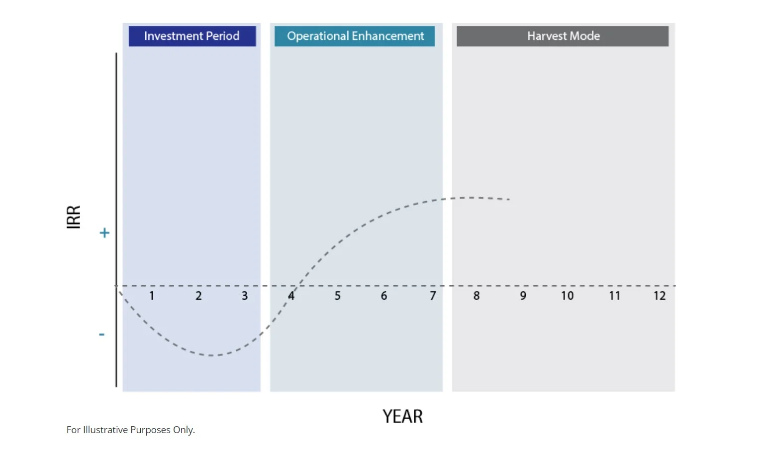
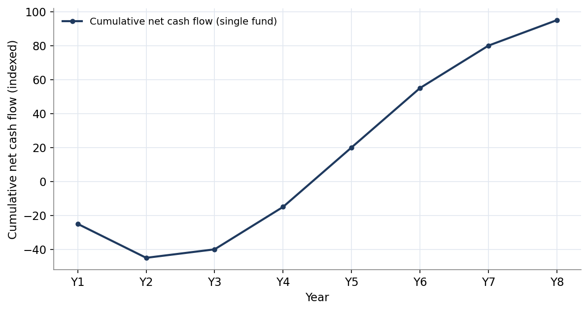
A private markets programme has an awkward shape in its early years. When a family office commits to a private markets fund, the fund does not take all the capital at once; it calls the capital over several years as it makes investments, and it charges fees from the outset, so the family office pays out capital and fees before the investments mature and return cash. The cumulative cash flow is therefore negative in the early years, reaching a trough, before the investments mature and distribute, turning the cash flow positive and tracing the shape of a letter J. This J-curve is the central liquidity challenge of building a private markets programme.
The J-curve matters because a family office must fund the capital calls when they come, and the calls are uneven and partly unpredictable, while the distributions that would offset them lag in the early years. A family office that has not planned for this can be caught short, unable to meet a call without selling other assets or scrambling for liquidity, or, at the other extreme, can hold so much idle cash against the calls that it drags the return of the whole portfolio. Managing the J-curve, the liquidity and the pacing of the programme, is therefore essential to building a private markets allocation without strain or drag.
This paper sets out a framework for managing the J-curve. The central argument is that the J-curve is managed not by avoiding it, which is impossible, but by pacing commitments across vintages to smooth it, by sizing liquidity buffers to meet calls through a stress, and by using financing tools to bridge the timing gaps. A family office that paces its commitments steadily, holds appropriate buffers, and uses the available tools builds its programme smoothly to target, while one that commits in bursts, holds inappropriate buffers, or lacks the tools faces liquidity strain or allocation drift. The J-curve is a manageable challenge, and managing it well is part of building a private markets programme.
The Commitment-Pacing Model
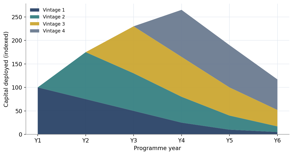
The commitment-pacing model is the central tool for managing the J-curve, smoothing the programme by committing steadily across vintages, illustrated in Figure 3. By committing a portion of the target allocation each year, the family office builds the programme across vintages, so that as the programme matures, earlier vintages distribute while later vintages call, the J-curves overlapping and partly offsetting to smooth the aggregate cash flow. The pacing model determines how much to commit each year to build the programme to target while smoothing the cash flow.
Figure 3. Commitment Pacing Across Vintages
The pacing model accounts for the fact that committed capital is called and returned over time, so the family office must commit more than its target allocation over the build period to reach and maintain the target invested allocation, because at any moment some commitments are not yet called and some capital has been returned. The model calculates the commitment pace that builds the invested allocation to target and maintains it, accounting for the calls, the distributions, and the re-investment of distributions into new commitments, which sustains the programme at target once built.
Once the programme reaches its target, the pacing model sustains it by committing each year an amount that replaces the capital being returned by maturing vintages, maintaining the target allocation as a rolling programme. The mature programme is self-sustaining in its pacing: the distributions from maturing vintages fund new commitments, and the steady pacing maintains the target allocation and the smooth cash flow. The pacing model therefore both builds the programme to target and sustains it, and it is the central tool for managing the J-curve across the programme life.
The pacing model should be adjusted for the family office liquidity position and risk tolerance, pacing faster to reach target sooner where liquidity is ample, more cautiously where liquidity is tight, as the decision framework in Figure 8 illustrates. A family office with ample liquidity can pace faster, even over-committing as examined in Section 10, to reach target sooner, while one with tight liquidity should pace cautiously to protect its liquidity. The pacing model is therefore tailored to the family office liquidity position, balancing the speed of reaching target against the liquidity risk, which the framework structures.
Liquidity Buffers
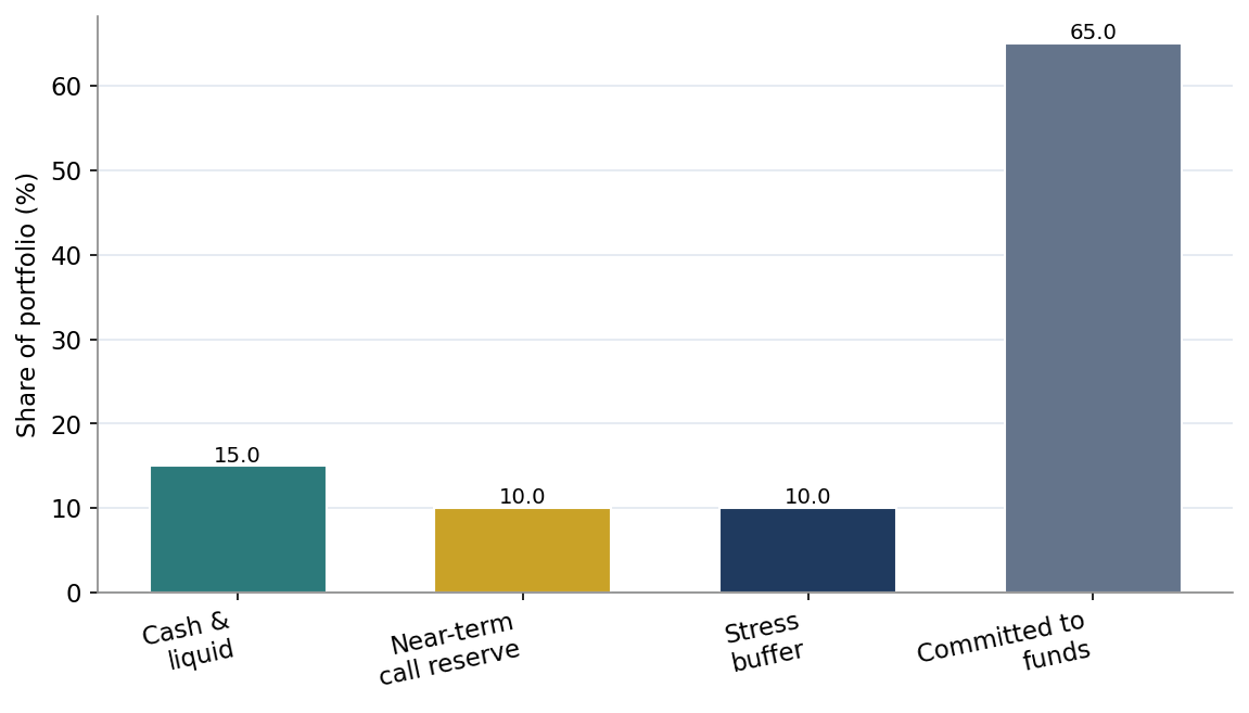
Managing the J-curve requires the family office to hold liquidity buffers to meet the capital calls, including through a stress, illustrated in Figure 6. The family office should hold a buffer of cash and liquid assets sufficient to meet the expected calls, plus a reserve for the unpredictability of the calls, plus a stress buffer for the possibility that distributions slow and calls continue in a downturn. The buffers ensure the family office can meet its calls without being forced to sell other assets or scramble for liquidity, which is the core of managing the J-curve liquidity.
Figure 6. Liquidity Buffers for a Private Markets Programme
The buffers must be sized to balance two risks: too small a buffer risks being caught short when calls come, particularly in a stress when distributions slow, while too large a buffer holds excessive idle cash that drags the return of the whole portfolio. The family office should size the buffers to meet the expected and stressed calls without excessive idle cash, which requires modelling the calls and distributions, including under a stress, to determine the buffer needed. The buffer sizing is therefore a balance, informed by the cash-flow modelling examined in Section 12, between the liquidity risk and the return drag.
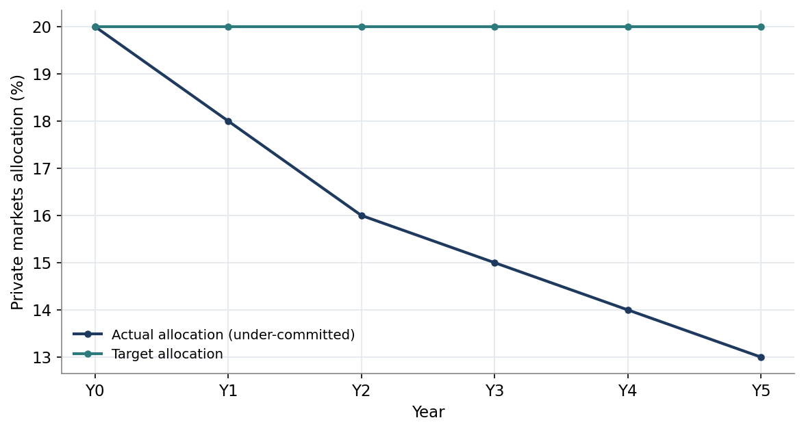
The stress buffer is particularly important because the J-curve liquidity challenge is greatest in a downturn, when distributions slow, extending the period of negative cash flow, while the denominator effect may also push the allocation above target. A family office that holds a stress buffer can meet its calls through a downturn without forced selling, while one that holds only an expected-case buffer may be caught short when distributions slow. The stress buffer is therefore the protection against the downturn scenario that most stresses the J-curve liquidity, and sizing it for a realistic stress is essential to managing the programme through the cycle.
Risk Management: Liquidity Stress
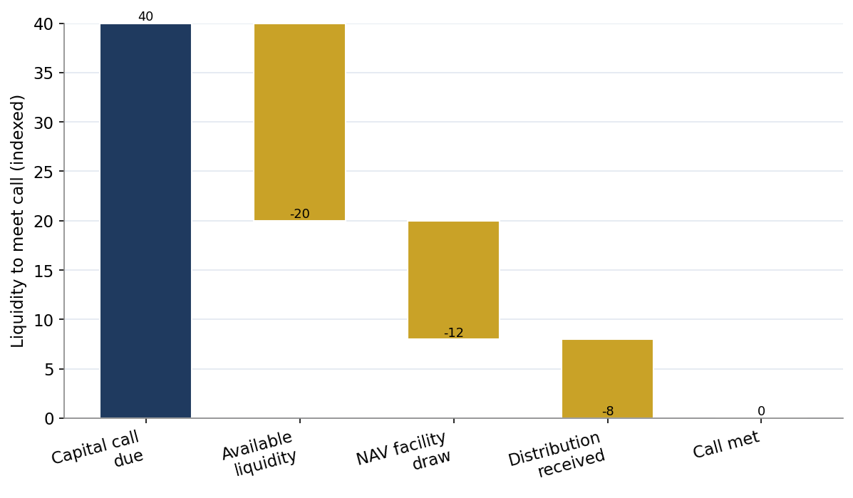
The principal risk in managing the J-curve is a liquidity stress, in which capital calls continue while distributions slow, typically in a downturn, leaving the family office struggling to meet its calls. This stress is the scenario the liquidity buffers and tools must cover, and managing it is the core of the J-curve risk management. A family office that plans only for the expected case, with calls and distributions as forecast, may be caught short in the stress, when distributions slow and the net liquidity demand rises, which is why the stress scenario must be planned for explicitly.
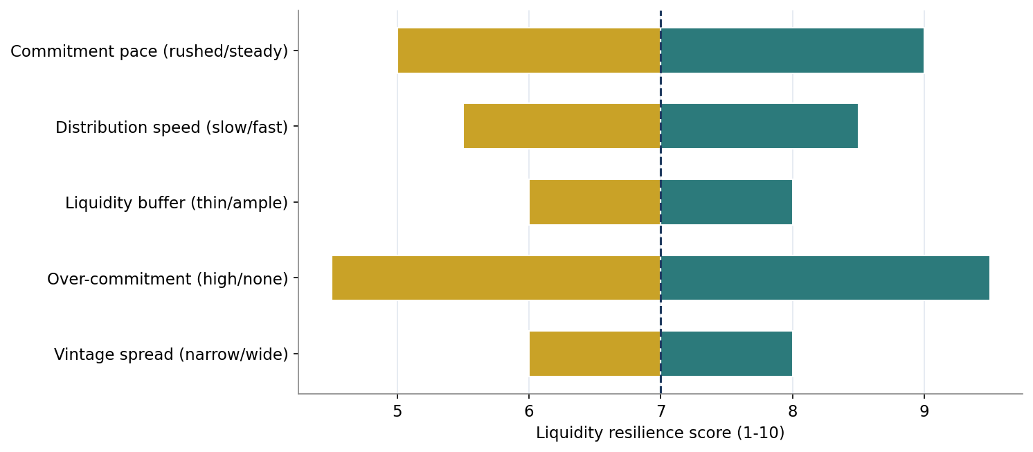
The stress is exacerbated by the denominator effect and over-commitment, which can compound in a downturn: public markets fall, pushing the private markets allocation above target through the denominator effect, while distributions slow and calls continue, and any over-commitment adds to the calls, straining the liquidity. A family office that has over-committed and holds a thin buffer can face a severe liquidity strain in this compound stress, forced to sell assets at depressed prices or default on a call, which is the danger the framework warns against. The risk management must therefore plan for this compound stress, sizing the buffer and limiting the over-commitment to survive it.
Managing the stress requires the stress buffer examined in Section 9, sized to meet the calls through a realistic downturn when distributions slow, plus the financing tools examined in Section 11, which provide a backstop liquidity, plus a prudent over-commitment that does not exceed the family office capacity to fund the calls through the stress. A family office that holds a stress buffer, has access to financing tools, and limits its over-commitment can meet its calls through the stress without forced selling, while one that holds a thin buffer, lacks the tools, and has over-committed may be caught short. The combination of buffer, tools, and prudent over-commitment is the stress management.
Case Studies
Three family-office cases illustrate the framework applied to different liquidity positions. The figures are modelled for analytical clarity and are not drawn from any specific family office.
Case A: the cautious family office
Case A is a family office with a measured liquidity position that paces its private markets build cautiously, committing steadily across vintages without over-committing, and holding ample liquidity buffers. It reaches its target allocation more slowly, over several years, but it manages the J-curve with little liquidity stress, meeting its calls comfortably from its buffers and the smoothed cash flow of its diversified vintages. The case illustrates the cautious approach, prioritising liquidity safety over speed of reaching target, suiting a family office that values liquidity security.
Case B: the balanced family office
Case B is a family office with a balanced liquidity position that paces its build steadily across vintages, with a modest over-commitment to reach target efficiently, and holds appropriate buffers supplemented by financing tools. It reaches its target allocation at a reasonable pace, manages the J-curve through its diversified vintages, buffers and tools, and maintains a balanced liquidity position. The case illustrates the balanced approach, reaching target at a reasonable pace while managing the J-curve liquidity with buffers and tools, suiting a family office balancing speed and liquidity safety.
Case C: the over-committing family office
Case C is a liquidity-rich family office that paces its build faster, over-committing to keep its programme fully invested and reach target sooner, relying on its ample liquidity, its distribution flow, and financing tools to meet the calls. It reaches its target allocation quickly and keeps its programme fully invested, but it bears a higher liquidity stress risk if calls coincide in a downturn, which its ample liquidity and tools are sized to cover. The case illustrates the over-committing approach, reaching target quickly from a position of liquidity strength, suiting a liquidity-rich family office that can bear the higher stress risk.
Figure 8. Time to Target and Liquidity Stress Risk by Approach
Common Errors and How to Avoid Them
A recognisable set of errors recurs in managing the J-curve.
Bursty commitment. Committing in concentrated bursts rather than steadily across vintages deepens the J-curve and concentrates the calls and the cycle risk. The remedy is steady pacing across vintages.
Under-committing. Committing only the target allocation, ignoring the gap between committed and invested capital, under-builds the programme. The remedy is to size commitments to reach target, accounting for the gap.
Excessive over-commitment. Over-committing beyond the liquidity capacity risks a strain or default when calls coincide in a downturn. The remedy is to size over-commitment to the stress capacity.
Thin buffer. Holding a thin buffer that does not cover a stress risks being caught short when distributions slow. The remedy is a stress buffer plus financing tools.
Over-reacting to drift. Over-reacting to the denominator-driven allocation drift in a downturn can lead to under-committing in attractive vintages. The remedy is a measured view of the drift.
Each of these errors is avoidable through the disciplined approach the framework encourages: pace steadily across vintages, size commitments to reach target, limit over-commitment to the stress capacity, hold a stress buffer with financing tools, and take a measured view of the drift. The family office that does so builds its programme smoothly to target and manages the J-curve liquidity through the cycle, while the one that does not faces a deep J-curve, under-builds, over-commits, holds a thin buffer, or over-reacts to drift. The discipline is what manages the J-curve from a challenge into a manageable feature of the programme.
Implementation Roadmap
Model the expected and stressed cash flows, the calls and distributions, across the programme, as the analytical foundation for the liquidity planning.
Pace commitments steadily across vintages, building the vintage diversification that smooths the J-curve and diversifies the cycle.
Size commitments to reach and maintain the target allocation, accounting for the gap between committed and invested capital and the re-investment of distributions.
Hold liquidity buffers sized to meet the calls through a realistic stress, balancing the liquidity risk against the return drag.
Use over-commitment only within the liquidity capacity, sized to fund the calls through a stress, and only for a mature, liquidity-rich programme.
Build access to the financing tools, NAV facilities, credit lines and the secondary market, to bridge calls and manage the liquidity efficiently.
Build the liquidity-management capability, the modelling, pacing, buffers and tools, and manage the programme actively through the cycle.
Conclusion
The J-curve, the early negative cash flow of a private markets programme before distributions catch up, is the central liquidity challenge of building a private markets allocation, and managing it well is essential to building the allocation without strain or drag. This paper has shown that the J-curve is managed not by avoiding it but by pacing commitments across vintages to smooth it, sizing liquidity buffers to meet calls through a stress, using financing tools to bridge the timing gaps, and managing the over-commitment and the denominator-driven drift that complicate the build.
The central conclusions are that vintage diversification through steady pacing is the core technique for smoothing the J-curve; that commitments must be sized to reach target, accounting for the gap between committed and invested capital; that over-commitment keeps the programme invested but must be limited to the stress liquidity capacity; that the liquidity buffers and financing tools must cover a realistic stress; and that the liquidity management is the enabler of the whole private markets programme. The family office that builds the liquidity-management capability and manages the J-curve with the discipline the framework describes can build and sustain a substantial private markets programme through the cycle, and the frameworks in this paper are intended to help it do so.
Limitations and Directions for Further Research
This paper is framework-oriented and relies on modelled figures, and its conclusions are directional rather than precise. The cash-flow profiles, pacing models and buffer sizes are calibrated to observable conditions but are not empirical estimates, and they vary across funds, strategies and programmes. The behaviour of calls and distributions in a stress, central to the framework, is uncertain and varies across downturns.
Several extensions would strengthen the analysis. An empirical study of capital call and distribution patterns across funds and strategies would replace the modelled profiles with data. An analysis of how private markets programmes managed their liquidity through past downturns, when distributions slowed, would test the framework stress assumptions. And a study of the use and effectiveness of the financing tools, the NAV facilities, credit lines and secondaries, in managing the J-curve would illuminate their role. Each is a natural subject for a later paper in this series.
| Scenario | Over-commitment | Distributions | Resilience |
|---|---|---|---|
| Resilient | None / modest | Normal | High |
| Balanced | Modest | Normal | Good |
| Stressed | High | Slow (downturn) | Strained |
| Crisis | Excessive | Frozen | At risk of default |
