

1 Define the acquisition question before selecting the model
This paper develops an author-proposed acquisition-diligence framework. Its recommendations concern the analysis and presentation of evidence; published findings and provider statements are separately attributed. No target wind farm, forecast, acquisition price, electricity contract or lender term has been supplied for verification. The starting question is specific: which energy assumption is disputed, which forecast periods it affects and which transaction decision requires an answer.
Fuchs and colleagues explicitly connect uncertainty in flow and engineering models with the calculation of net production used for offshore-project financing. Their Gulf of Mexico study used FLORIS and a defined hypothetical layout. That statement supports attention to model uncertainty in energy assessment; the report's scope remains regional development analysis.[2] In the proposed transaction framework, the committee receives an energy question, an evidence question and a financial question as separately assigned tasks.
Three linked calculations organise that question. The physical calculation estimates production under a stated resource and plant configuration. The uncertainty assessment characterises the evidence and limitations around that estimate. The commercial calculation applies the relevant pricing, operating and financing terms. An energy revision can therefore enter several financial lines, each requiring its own calculation. The committee needs the physical case and its commercial transmission before approving a bid adjustment.
Operating and development acquisitions begin with different available evidence. An operating-farm assessment can reconcile metered production with the installed configuration and recorded operating states. A development assessment can examine measured resource, proposed design and documented neighbouring projects. The evidence actually available determines which comparisons can be completed. Missing operating history remains a limitation in a development case; an assumed history cannot enter the evidence register.
A concise issue record connects the seller case, buyer case, changed inputs, unresolved disagreement and independent check. Its decision column states whether the issue affects the central forecast, the uncertainty range, a future-build-out scenario or several identified components. The committee sets the monetary threshold, timetable and approval authority for escalation. Those are transaction choices; the reviewed studies supply no universal acquisition threshold.
2 Reconstruct the evidence chain and preserve its definitions
IEC 61400-15-1:2025 addresses site-suitability input conditions for onshore and offshore plants. Its published scope covers long-term meteorological and wind-flow characteristics, integration with plant characteristics, environmental drivers and documentation traceability. The publicly available description supplies a basis for requesting a traceable assessment record. The paid standard's detailed clauses were not inspected for this paper.[1]
The evidence chain begins with the raw observation or authoritative design record. Each derived input needs its transformation, responsible party, version, units, time basis and applicable configuration. A resource file retains measurement height and location; a turbine file retains the power and thrust information used; a model run retains its software and settings. The relationship between these files is part of the analysis. A reviewer should be able to follow a reported energy figure back through each transformation.
Loss percentages require explicit denominators. For two sequential deductions defined as fractions of the quantity entering each step, the retained quantity is E0 multiplied by (1-l1) and (1-l2). A joint interaction calculation has its own counterfactual definition. These arithmetic conventions produce different bridges, so the calculation should show energy before and after every step. The method actually used determines the appropriate convention; the reviewer records that convention alongside the result.
Table 1. Proposed evidence-to-calculation register
| Evidence layer | Minimum record requested | Reconciliation question |
|---|---|---|
| Resource | Raw measurements, reference data, height and period | Which observations support each climate input? |
| Plant | Coordinates, installed specification, control versions | Which physical configuration does the run represent? |
| Flow model | Software, settings, calibration and output files | Can an authorised reviewer reproduce the result? |
| Loss accounting | Definitions, denominators and calculation sequence | Where does each deduction enter net export? |
| Forecast hand-off | Time-series output and case identifiers | Which technical case feeds each financial scenario? |
Author-proposed diligence requests. No asset evidence has been supplied.
The decision deliverable is a controlled case pack: input manifest, calculation bridge and exceptions log. Reproduction of a selected case tests the connection between the supplied files and the reported output. Licensing or data restrictions should carry the scope of the alternative review. Counsel separately checks reliance rights. A committee can then identify which technical conclusion is reproducible, which is independently reviewed and which still depends on unavailable information.
3 Examine internal wakes through turbine-level counterfactuals
An internal-wake estimate compares two defined energy quantities: production for a specified turbine arrangement and production in its reference configuration. If Eref is reference energy and Earray is array energy, a diagnostic loss fraction can be defined as (Eref-Earray)/Eref. That definition establishes the denominator and comparison boundary. Direction, wind-speed bin, turbine state and annual weighting then connect the diagnostic result to the reported forecast.
Cooperman and colleagues used FLORIS to compare generating potential across Humboldt and Morro Bay lease delineations. Their calculations considered turbine spacing, mooring assumptions and neighbouring arrays; the report also compares TurbOPark implementations.[3] This is a documented California example of configuration and model-version sensitivity. An acquisition review requires its own installed or proposed coordinates and turbine files.
A direction-resolved comparison localises a disagreement. The review checks the direction record, upstream operating state, turbine thrust and control specification, then tests whether the comparison retains the same sample after exclusions. A difference confined to one sector calls for investigation of that sector's inputs and coverage. A difference across the entire array calls for examination of shared inputs and model configuration. These are diagnostic routes; the target records determine their findings.
Operating-state treatment belongs inside the counterfactual definition. A run with all turbines available represents a different configuration from a run reproducing recorded outages or derating. A downstream power comparison needs the upstream states used in that same comparison. A diagnostic limited to selected turbines should identify those turbines and the permitted use of its result. The annual forecast reconciliation remains a whole-boundary calculation with its own coverage and weighting.
A directional reconciliation sheet gives the committee a decision record. It shows the seller case, reviewer case and controlled reruns, with one changed item in each diagnostic test. Retaining the annual total alongside the diagnostic subset identifies the financial relevance of the tested difference. A supported change can enter the forecast bridge; a restricted observation retains its restricted scope. No numerical internal-wake allowance is assigned to an unidentified asset.
4 Treat neighbouring development as dated scenario evidence
Porchetta and colleagues compare WRF with engineering models for the Princess Elisabeth and Belgian-Dutch clusters using meteorological year 2016. Their external-loss estimates have greater relative inter-model spread than internal-loss estimates, especially during summer. The study explicitly identifies the absence of validation ground truth within its scope.[4] This is a model-comparison finding for a defined southern North Sea setting.
An external-wake scenario adds another physical configuration to the comparison. The target farm is evaluated alone and with a specified neighbouring arrangement under matched resource inputs. The energy difference is conditional on that arrangement and its operating period. A dated register supplies the status, boundary, available layout and turbine specification of each included development. Missing designs remain missing; management proxy layouts carry that label. The study area needs an explicit inclusion criterion.
Table 2. Proposed external-build-out case register
| Case component | Evidence requested | Treatment proposed |
|---|---|---|
| Operating neighbour | Verified configuration and operating date | Reproduce documented configuration |
| Project under construction | Authoritative status and available design | Record supported timetable; identify open design items |
| Consented development | Consent, boundary and current sponsor information | Separate status evidence from management timing assumptions |
| Early-stage proposal | Dated public announcement and available rights information | Retain as a labelled sensitivity if committee requests it |
| Unknown design | Explicit list of missing inputs | Report unresolved exposure and any labelled proxy run |
No project statuses, commissioning dates or construction probabilities are assumed.
Timing enters through the period during which each configuration operates. The scenario pack pairs physical layouts with commissioning schedules and identifies the status date used. A cumulative case lists every included project. Management probabilities remain management estimates with an approver and date. The engineering output retains its conditional case label when those estimates enter a financial calculation. This separates the simulated consequence of build-out from management's assessment of whether and when it occurs.
The bid decision can respond separately to known configuration, timing exposure and unsupported design inputs. A dated baseline and change log show what has changed between indicative bid, final bid and completion. Each update should identify its effect on the approved physical case and the affected forecast years. Potential legal remedies require jurisdiction-specific advice and the relevant executed documents; the reviewed engineering studies establish no such entitlement.
5 Make stability and atmospheric inputs inspectable
Rosencrans and colleagues modelled a year of US mid-Atlantic offshore conditions with no-farm, single-farm and lease-area build-out cases. Their strongest simulated wakes extended 55 km during summer stable stratification. They tested turbine-added turbulent kinetic energy and reported non-additive combined internal/external effects. The authors expressly exclude commercial judgments about individual projects from the study's intended use.[5]
Porchetta and colleagues identify reduced mixing, slower wake recovery and greater sensitivity to recovery formulation under stable stratification as drivers of the spread in their comparison.[4] Atmospheric inputs therefore need inspectable definitions: stability variables, measurement or derivation, coverage and uncertainty treatment. A constant parameter represents a stated simplification. A time-varying input needs its source, resolution and transformation. The committee should see where the method extrapolates beyond available observations and which quantities depend on that extrapolation.
Annual weighting is part of this mechanism. A model result evaluated for a particular condition enters the annual estimate through the weight assigned to that condition. The review therefore needs a joint-coverage table for direction, speed, turbulence and the selected stability representation. Empty or thinly represented cells remain visible. Minimum sample rules and sensitivities require project-specific justification; the annual estimate should retain the coverage limitations of its component cases.
A controlled atmospheric comparison holds layout and turbine characteristics fixed and applies documented alternatives. Its output identifies the production change and observational support for each alternative. Measurement or classification uncertainty can be tested in a separate sensitivity. The result changes the decision in a specific way: a supported atmospheric-input correction enters the central bridge, while an unresolved modelling choice remains in the named scenario range. No probability attaches to an alternative without a documented method.
Different seller and reviewer atmospheric descriptions require their own reconciliation. The bridge identifies data periods, direction weights, turbulence treatment and the resulting change under each controlled rerun. An unexplained parameter difference remains unresolved in the investment paper. The final decision record states which atmospheric case management accepts and which residual sensitivities remain in underwriting. This makes the selected annual weighting and its evidence visible to the committee.
6 Review blockage at the same boundary as wake interactions
Carbon Trust's GloBE announcement describes a German Bight measurement campaign at Amrumbank West and Nordsee Ost, including scanning and floating LiDAR and instrumentation for atmospheric conditions. Its stated aim is a primary dataset for validating and improving models used in investment decisions.[11] The programme page records intended measurement and validation work; it supplies no asset-specific loss adjustment.
Blockage concerns the approaching flow and its diversion around a farm; GloBE explicitly investigates the upstream slowdown and acceleration elsewhere.[11] Its accounting requires a defined reference inflow and domain. An assessment combining wake and blockage in one interaction term should preserve that combined definition in the energy bridge. An assessment using separate terms needs documented interfaces, including any overlapping physical or computational treatment. The selected accounting boundary determines the comparison the committee receives.
A counterfactual map connects reference inflow, farm configuration, neighbouring configuration and calculation domain. Each reported difference identifies the changed configuration. The reference measurement location and spatial interpolation belong on that map. Where a resource input represents conditions influenced by existing farms, the assessment should explain its relationship to the subsequent interaction calculation. The review then has a defined route for examining overlap in the modelling chain.
Method changes can be examined through matched reruns using the same resource and layout files. The reconciliation decomposes the difference into input, software, parameter and remaining methodological changes to the extent computationally possible. An inseparable component retains that limitation. The decision is then based on the established net difference and documented explanation. An attributed provider claim about a new method remains separate from the reviewer's evidence for the target.
Historical budgets, the current operating budget and the acquisition forecast should each retain a dated methodology identifier. A transition enters the decision log with its documented reason and authorised effect on the forecast. This identifies the case that supports the bid and the bridge from earlier cases. A generic blockage percentage from another geography remains outside this framework's evidence standard; any target allowance requires its own supported calculation.
7 Build an auditable SCADA cleaning and reconciliation record
Mittelmeier, Blodau and Kühn demonstrate offshore performance monitoring using turbine states, wake-model lookup tables and expected-versus-measured power ratios. They assess uncertainty and demonstrate detection of degradation and curtailment. Their study provides a specific monitoring method and application, including a triple-wake example; any target review needs its own documented applicability test.[9]
SCADA analysis begins with an untouched inventory of received files, coverage, clocks, units, turbine identifiers and status-code definitions. Each processed record retains its relationship to the original and its retained, excluded or transformed state. Exclusion counts by turbine, month and reason describe the sample that supports the result. The script or reproducible configuration supplies the analytical record. A reported power relationship should therefore travel with its data selection.
Table 3. Proposed operating-data processing controls
| Processing issue | Record requested | Check proposed |
|---|---|---|
| Time basis | Source clocks, time zones and interval definitions | Match records using a documented conversion |
| Operating states | Status dictionary, dispatch and maintenance records | Preserve the reason for each inclusion or exclusion |
| Sensor quality | Calibration, replacements and diagnostic records | Label corrected values and retain originals |
| Missing records | Gap map and any reconstruction method | Separate measured and reconstructed quantities |
| Plant export | Revenue meter and electrical boundary definition | Reconcile turbine totals through identified differences |
Author-proposed controls; thresholds and classifications require target-specific evidence.
Filtering changes the population being analysed. A calculation restricted to normal operation measures performance within that selected state; a calculation using the entire history addresses a different observed quantity. Alternative-filter sensitivities should retain the same diagnostic definition and report both coverage and the resulting metric. Each exclusion rule needs an engineering explanation or recorded analytical rationale. A rule introduced after result inspection requires a dated reason and approver.
The production reconciliation follows quantities through documented boundaries: turbine records, plant electrical systems and revenue-meter export. Every residual difference needs an identified explanation or an unresolved-item label. A missing-record reconstruction carries its method and qualification. The committee receives the operating evidence and the forecast derived from it as linked outputs, with units and periods explicit. It can then decide whether an apparent discrepancy supports a forecast change, additional analysis or an open diligence item.
8 Distinguish operating reconciliation from long-term normalisation
DNV's operational-energy service description covers the use of operating data for P50/P90 estimates, corrections for long-term efficiency and availability, correlation to wind measurements and optional uncertainty analysis.[14] This is an attributed service description. The present paper has no target operating assessment or independent verification of a provider's result.
Operating reconciliation accounts for the supplied records over their actual period. Long-term normalisation applies a documented method to represent the forecast period. The two calculations have distinct purposes and separate bridges. Reference datasets, concurrent periods, correlation methods, exclusions and their uncertainty treatment belong in the normalisation bridge. A shared production boundary supports comparison; any boundary change needs its own reconciliation. The reader can then distinguish an observed-period discrepancy from an adjustment to future expectations.
A regime log identifies commissioning stages, replacements, control changes, material repairs, measurement changes and neighbouring commissioning from dated records. Normalisation across these regimes requires an explicit comparability assumption or a separately modelled configuration. Incomplete records leave particular boundaries unverified. This is a decision-relevant limitation: the committee needs to know which operating configuration supplies the evidence for the acquired plant and which adjustments are required to reach it.
Calibration and evaluation records should have separately identified roles. The analysis states how their split was selected, which adjustments used each subset and which periods remain unused. Seasonal and directional coverage describes the evidence actually available. A forecast based on a limited record should retain those coverage qualifications. The decision record can then distinguish a result reproduced during model development from a result evaluated using separately identified evidence.
A neighbouring farm's verified commissioning supplies a dated configuration change. The normalisation method should explain how both the reference series and target series represent it. Each correction needs its equation, input source and comparison against available observations. An unverifiable correction remains a labelled assumption. The committee's deliverable is an observed-period account and an identifiable long-term adjustment schedule, including the unverified inputs management has chosen to retain.
9 Separate model inadequacy, parameter uncertainty and scenario choice
Aerts, Devesse and Meyers develop a Bayesian framework separating model inadequacy from measurement uncertainty and estimating model parameters. Their demonstration uses large-eddy simulations of blockage and atmospheric gravity waves in conventionally neutral boundary layers. Omitting model inadequacy produces overly confident posterior estimates in that exercise.[6] Its reference evidence is simulated; a target's operating-data calibration requires separate substantiation.
An uncertainty register gives each term a definition, unit, estimator, supporting dataset and owner. Measurement error, parameter estimation, model inadequacy, long-term adjustment and future configuration have separately stated roles. A set of scenario outputs retains its case labels until a probability treatment has been documented. Dispersion between selected models can be reported directly as dispersion. Converting it into a probability distribution requires an additional method and supporting assumptions.
For a linear combination X of components Xi with fixed weights ai and finite variances, variance is the sum of ai squared times each component variance, plus twice the sum of weighted covariances across distinct component pairs. This identity explains why dependence belongs in an uncertainty budget. A dependency map identifies shared records, direction corrections, turbine inputs and calibration evidence. The assessment states which dependencies are represented and which remain unquantified. No project covariance coefficient is assumed here.
Expected losses and uncertainty around those losses also need separate entries. Each forecast adjustment should identify its purpose and position in the calculation bridge. A downside case states its changed inputs and accompanying uncertainty treatment. Where a base-case adjustment and another allowance concern the same finding, their combined treatment needs reconciliation. The committee can then approve the expected production case and the retained uncertainty treatment as identifiable decisions.
Every probabilistic output used by the committee needs a named quantity, forecast horizon and calculation method. The central estimate, distribution and exceedance metric should connect through a reproducible calculation. Their changes can then be reported separately: a revised central case, revised dispersion or both. The downstream financial model receives those distinct changes with their stated interpretation. This paper assigns no P90 haircut or distribution shape to an unidentified asset.
10 Compare models with matched questions and geographic limits
The AWAKEN benchmark involved 16 research groups and a diurnal onshore case. Its interpretation explicitly addresses differences in inflow information supplied to models; refinements using richer observations are state-conditioned.[7] Elizalde and colleagues examine North Sea regional scenarios with COSMO6.0-CLM, varying forcing, turbine choices and wake parameterization. Their approximately 10% quantity is relative to installed capacity in a 150 GW scenario.[8]
Model comparisons answer a specified question: software implementation, calibrated parameters, physical formulation or the full assessment workflow. A controlled comparison matches layouts, turbine specifications, meteorological periods and reporting boundaries. An operational comparison may retain each provider's chosen workflow, with its distinct inputs documented. The interpretation follows the comparison actually performed. Unavoidable differences belong in a manifest and, where practicable, in a controlled sensitivity explaining their contribution.
Table 4. Verified examples and the limits of transaction transfer
| Source example | Evidence scope | Limit to retain |
|---|---|---|
| California leasing assessment[3] | Layout and model sensitivities | Hypothetical delineations and technology assumptions |
| Southern North Sea comparison[4] | WRF versus engineering predictions | Inter-model spread; ground truth unavailable in study |
| US mid-Atlantic study[5] | Yearlong offshore build-out simulations | Defined regional scenarios |
| AWAKEN benchmark[7] | Onshore diurnal field benchmark | Inflow information and case conditioning |
| North Sea regional scenarios[8] | Forcing, turbine and parameterization variation | Regional capacity-based result |
Source scopes are verified; transaction applications require target-specific evidence.
Evaluation should state the predicted quantity and the residual metric. Direction-resolved and operating-state-resolved diagnostics retain their sample counts and applicable configuration. An annual total retains its component coverage and weighting. A metric averaged over a period answers that period's defined question. A forecast revision requires a documented connection to the target forecast, including the method used to carry regime-level results into annual production.
Implementation checks, agreement with independent measurements and agreement with another model should retain their own result labels. Shared inputs and training or reference simulations belong in the comparison record. The selection rationale then states which test supports the preferred method for the target question. Geography, plant scale, atmospheric regime and evaluation period remain explicit limits. The committee approves a method together with those limits and any additional evidence required.
11 Apply explicit validation gates to AI-assisted assessments
DNV describes CFD.ML as a machine-learning interaction model trained on high-fidelity WRF-to-CFD simulations, predicting wake and blockage together. Its public page reports a roughly 30-farm blind comparison against a CFD reference and states offshore-assessment implementation from 1 June 2026.[13] These are DNV's published statements. The gated full whitepaper was not accessed, and independent field-validation evidence was not verified for this paper.
A learned surrogate's evidence chain includes both its training reference and its evaluation evidence. The review therefore needs the training-domain description, target-domain comparison, release history, applicable input ranges and reference physics. Inputs outside the stated evaluation domain require a documented treatment. Proprietary restrictions should have a clear effect on the scope of independent review. Unavailable information remains a limitation in the committee's reliance decision.
Three evaluation gates organise that evidence. Implementation testing examines whether the supplied configuration runs as documented. Surrogate-reference testing compares outputs with the stated computational reference. Field-evidence testing compares permitted outputs with independent measurements under documented conditions. Each gate has a separate result and limitation. Agreement at one gate supplies evidence for that stated test; the acquisition review should identify the additional evidence used for the remaining questions.
Model governance records calibration and evaluation separation, project overlap between datasets, revisions after evaluation and release approval. Error metrics should retain atmospheric and layout regimes relevant to the target, together with sample counts. A general provider accuracy statement remains attributed where these details are unavailable. The committee's choice is then explicit: the supported scope of use, the evidence still required and the residual limitations accepted in underwriting.
The agreed acquisition baseline should identify a frozen release. A later version enters the change log with a controlled rerun and explanation of changed outputs. Acceptance records what was tested, against which reference and within which scope. This creates a defined hand-off to post-acquisition monitoring and any later reassessment. No independent conclusion about improved target-farm yield estimation through AI-assisted prediction is established in this paper.
12 Carry the wake scenarios into hourly revenue calculations
The Gulf of Mexico report notes that a production effect and its revenue effect can differ with local electricity-price dynamics.[2] Carbon Trust describes reduction of loss uncertainty and improved bankability as OWA workgroup objectives.[12] Its Dublin Bay report calculates a hypothetical P90/P50 increase from 90.9% to 91.3% through improved spatial measurement, holding other uncertainty terms fixed.[10] These statements supply context; they establish no acquired asset's revenue, financing saving or debt capacity.
The financial hand-off retains the production time series for each approved technical case. In a simple energy-sale calculation, revenue R equals the sum of sold quantity qt multiplied by applicable price pt at each settlement interval t. Under unchanged prices, the difference between two cases is the sum of their interval quantity differences multiplied by pt. This arithmetic identifies the required hourly or settlement-period comparison. Executed pricing provisions determine the actual contractual calculation.
Annual energy totals alone do not specify that interval sum; it also requires the timing of quantity and price. Matched scenarios should therefore retain the production boundary, clock conversion, missing intervals and treatment of export constraints. Changes in dispatch, curtailment or price assumptions require their own identification. A controlled case can hold commercial inputs fixed to calculate the isolated effect of a technical scenario under those defined inputs.
Merchant-price inputs need a source and status: observed series, contracted provision, third-party forecast or labelled management estimate. Forward extrapolations retain their owner and date. Contracted and uncontracted quantities reconcile to the relevant agreements. Fees, imbalances and other settlement items enter only with a documented contractual basis or an explicitly labelled assumption. The committee can then distinguish the energy-model consequence from the commercial forecast it has approved.
The technical-to-financial schedule records gross production, modelled interactions, other documented adjustments, net export and settlement quantity by case and period. Finance applies the approved commercial inputs and retains the resulting cash-flow calculation. Debt sizing and acquisition value require additional supplied terms. The decision at this stage is the approved production-to-revenue bridge and its open items. A case can then reach the valuation workstream with its physical definition, commercial assumptions and limitations intact.
13 A finite-life acquisition model with explicit assumptions
Hypothetical illustration. Every asset characteristic, financial input, uncertainty assumption and transaction term in Sections 13-17 is invented for this worked example. The calculations describe a 500 MW wind farm operating for 20 years. They provide a transparent connection between energy assumptions, operating enterprise value and acquisition funding. They provide no valuation of an identified asset.
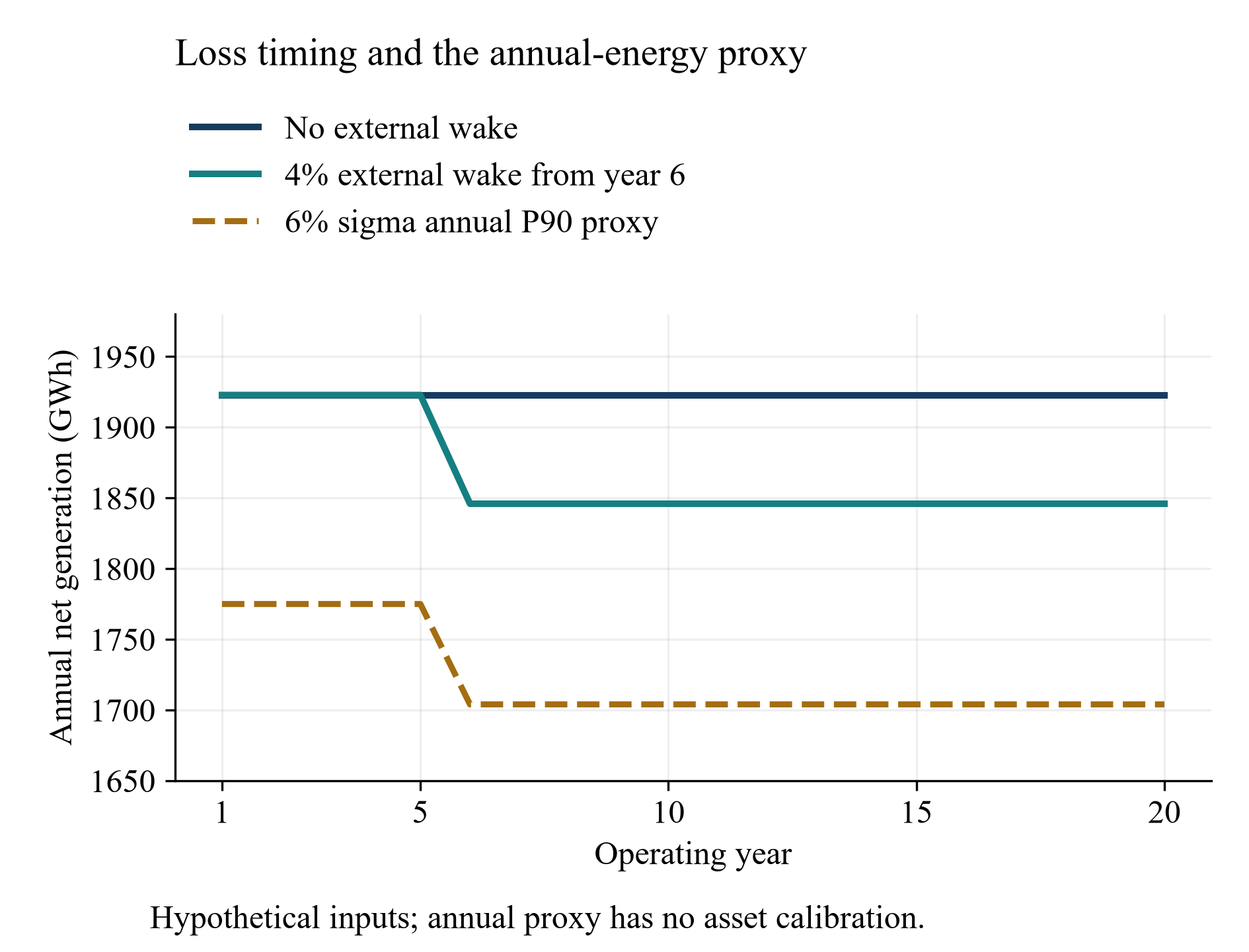
The model assumes gross annual generation of 2,200 GWh. Internal wake loss is 8%; other losses are 5%; the base case has zero external wake. Each loss factor applies to the energy remaining after the preceding factors. The resulting base net generation is 1,922.8 GWh. This convention gives a combined internal-wake-and-other reduction of 12.6%. Adding the percentages would produce a different energy estimate.
Equation 1.
Here, E is annual net generation in MWh; G is gross generation; the three loss fractions refer to internal wake, external wake in year t, and other losses. External-wake scenarios apply a further 2%, 4% or 6% reduction beginning in the specified year. The assumed loss is constant thereafter. This stylised timing represents a specified scenario; no neighbouring project's consent, commissioning date or engineering effect is asserted.
Table 5. Inputs to the hypothetical finite-life model.
| Input | Assumed value |
|---|---|
| Capacity; operating life | 500 MW; 20 years |
| Gross generation | 2,200 GWh/year |
| Internal wake; other losses | 8%; 5%, multiplicative |
| External-wake cases | 0%, 2%, 4%, 6% |
| Captured price; variable OPEX | EUR70/MWh; EUR3/MWh |
| Fixed OPEX; maintenance capex | EUR25m/year; EUR5m/year |
| Discount rate; terminal value | 8% real; zero |
| Central annual-energy sigma | 6% |
| Debt tenor; rate; proxy DSCR | 10 years; 5.5% real; 1.4x |
| Existing net debt; simplified tax | EUR100m; zero |
Hypothetical assumptions throughout; cash flows occur at year-end; EUR amounts are real; no asset calibration.
Captured price is fixed at EUR70/MWh, with EUR3/MWh variable operating expense. Fixed expense and maintenance capital expenditure total EUR30 million annually. Cash flow available for debt service, abbreviated CFADS, therefore equals net MWh multiplied by the EUR67/MWh contribution margin, less EUR30 million. The base annual CFADS is EUR98.8276 million. Tax is simplified to zero; no tax shield is included.
Equation 2.
P denotes captured price, v variable expense per MWh, F fixed expense and K maintenance capex. The same operating cash flow supplies the pre-tax, unlevered valuation. Figure 1 shows the generation profile and the separate annual-energy screening proxy discussed in Section 16.
View figure at full size; scroll horizontally on smaller screens.
Hypothetical: 500 MW; multiplicative losses; 4% external wake begins in year 6; central annual sigma 6%.
14 External-wake size and timing change operating value
Hypothetical illustration. Operating enterprise value is the present value of 20 annual operating CFADS amounts. The base discount rate is 8% real. There is no terminal value, perpetual extension or residual-value assumption. The calculation gives base operating EV of EUR970.3 million.
Equation 3.
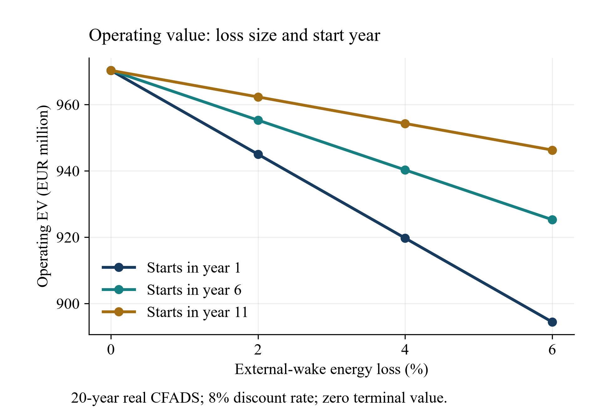
The discount rate r applies to end-year cash flows. A 4% external-wake loss beginning in year 6 reduces annual generation after that date to 1,845.888 GWh. The annual operating cash-flow reduction is EUR5.153104 million. Discounting that reduction over years 6-20 gives an operating-value loss of EUR30.0 million and scenario EV of EUR940.3 million. Fixed operating costs and maintenance capex remain unchanged.
Table 6. External-wake sensitivity from year 6.
| External wake | Net GWh | Operating EV, EURm | EV loss, EURm | Debt capacity, EURm |
|---|---|---|---|---|
| 0% | 1,922.800 | 970.3 | 0.0 | 478.8 |
| 2% | 1,884.344 | 955.3 | 15.0 | 473.2 |
| 4% | 1,845.888 | 940.3 | 30.0 | 467.7 |
| 6% | 1,807.432 | 925.3 | 45.0 | 462.1 |
Entirely hypothetical; 8% real discount rate; central sigma 6%; EURm figures rounded to one decimal. Generation is annual net energy after external wake begins.
Timing matters because it changes the number and present value of affected operating years. The assumed 4% loss beginning immediately produces EUR50.6 million of lost operating value. The same loss beginning in year 11 produces EUR16.0 million of lost operating value. These outcomes follow directly from the finite cash-flow schedule; no probability is attached to any start date.
Table 7. Timing sensitivity for the same 4% external-wake loss.
| First affected year | Operating EV, EURm | EV loss, EURm | Debt capacity, EURm |
|---|---|---|---|
| 1 | 919.7 | 50.6 | 453.1 |
| 6 | 940.3 | 30.0 | 467.7 |
| 11 | 954.3 | 16.0 | 478.8 |
Entirely hypothetical; 8% real discount rate; central sigma 6%; debt amortises over years 1-10.
The year-11 scenario retains base initial debt capacity because the assumed lender calculation uses years 1-10 only. It still reduces the operating value of the subsequent cash flows. Figure 2 displays both the size and timing dimensions, supporting explicit scenario discussion in an acquisition model.
View figure at full size; scroll horizontally on smaller screens.
Hypothetical 20-year real cash flows discounted at 8%; financing capacity is calculated separately.
15 The financing bridge and the closing equity requirement
Hypothetical illustration. Debt capacity is sculpted to an assumed 1.4x coverage ratio using the annual-energy P90-proxy CFADS. Debt service in each of years 1-10 equals that CFADS divided by 1.4. The opening loan equals the present value of those debt services at an assumed 5.5% rate. Its amortisation schedule repays the opening balance by year 10. These are chosen model terms; they establish no lender norm or available financing offer.
Equation 4.
D is opening debt capacity; i is the assumed debt rate. Debt pricing is expressed in real terms for consistency with the simplified real operating cash flows. Inflation and nominal debt service would require a separate nominal specification. Reserve accounts, financing fees and debt break costs are omitted.
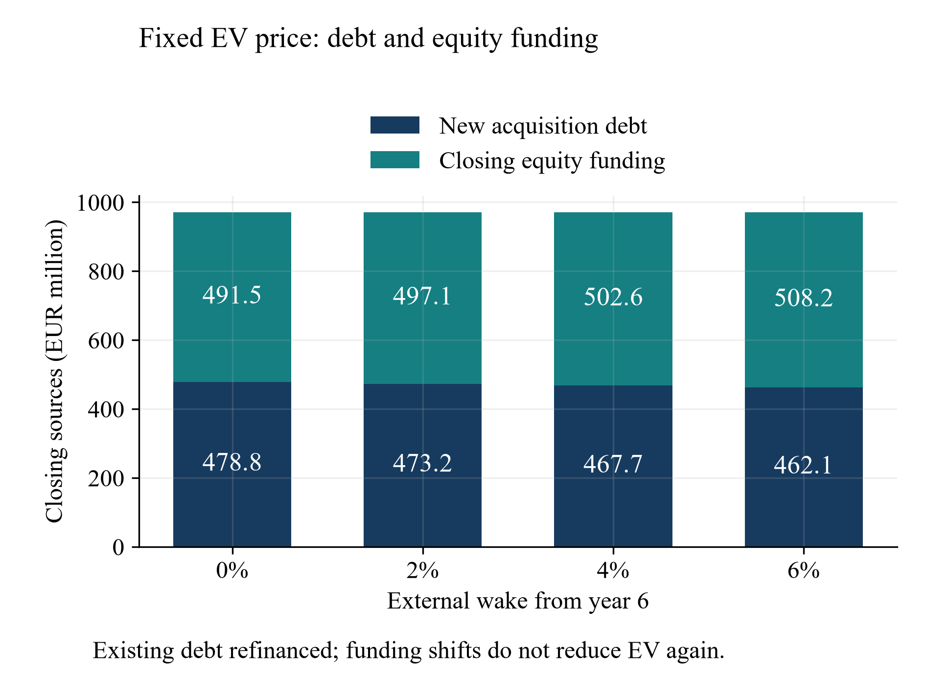
The transaction example holds enterprise-value purchase funding at the base seller reference of EUR970.3 million. Existing net debt of EUR100 million is assumed repaid or refinanced at closing. Seller equity consideration is consequently EUR870.3 million. New acquisition debt funds part of the total EV purchase requirement; closing equity funds the balance. The seller's share consideration and the purchaser's equity funding cheque are separate quantities.
Table 8. Operating valuation and acquisition-funding bridge.
| Quantity | Base | 4% wake case | Change |
|---|---|---|---|
| Model operating EV | 970.3 | 940.3 | -30.0 |
| Model equity value after existing debt | 870.3 | 840.3 | -30.0 |
| Fixed agreed purchase EV | 970.3 | 970.3 | 0.0 |
| Seller equity consideration at fixed EV | 870.3 | 870.3 | 0.0 |
| New acquisition debt capacity | 478.8 | 467.7 | -11.1 |
| Closing acquisition equity funding | 491.5 | 502.6 | +11.1 |
Entirely hypothetical; 4% external wake begins in year 6; fixed purchase EV is unchanged; existing EUR100m net debt is refinanced; all values EURm.
The EUR30.0 million operating-value reduction already reflects lost operating cash flows. The EUR11.1 million capacity reduction reallocates the funding of the unchanged price toward equity. The model carries no additional EUR11.1 million deduction from operating EV. A sponsor-return analysis would need the resulting debt-service schedule, distributions, fees and exit assumptions. No equity IRR is claimed here. Paying the unchanged reference price also leaves an unlevered value shortfall in the assumed wake case; the funding illustration supplies no endorsement of that price.
View figure at full size; scroll horizontally on smaller screens.
Hypothetical fixed EV reference equals base operating EV; existing debt is refinanced; the source mix changes as acquisition debt capacity changes.
16 Annual uncertainty, correlation and the P90 proxy
Hypothetical illustration. The central annual-energy proxy applies a standard-normal haircut using annual sigma of exactly 6% and a 90th-percentile z-value of approximately 1.28155. Proxy energy is approximately 92.31% of expected annual energy. The proxy CFADS then pays the same fixed operating expense and maintenance capex.
Equation 5.
This is a deterministic annual-energy screening convention. The model has no asset-calibrated exceedance probability, multi-year joint distribution or explicit inter-year dependence. It provides no calibrated 20-year P90 statement. The normal approximation is also a chosen simplification.
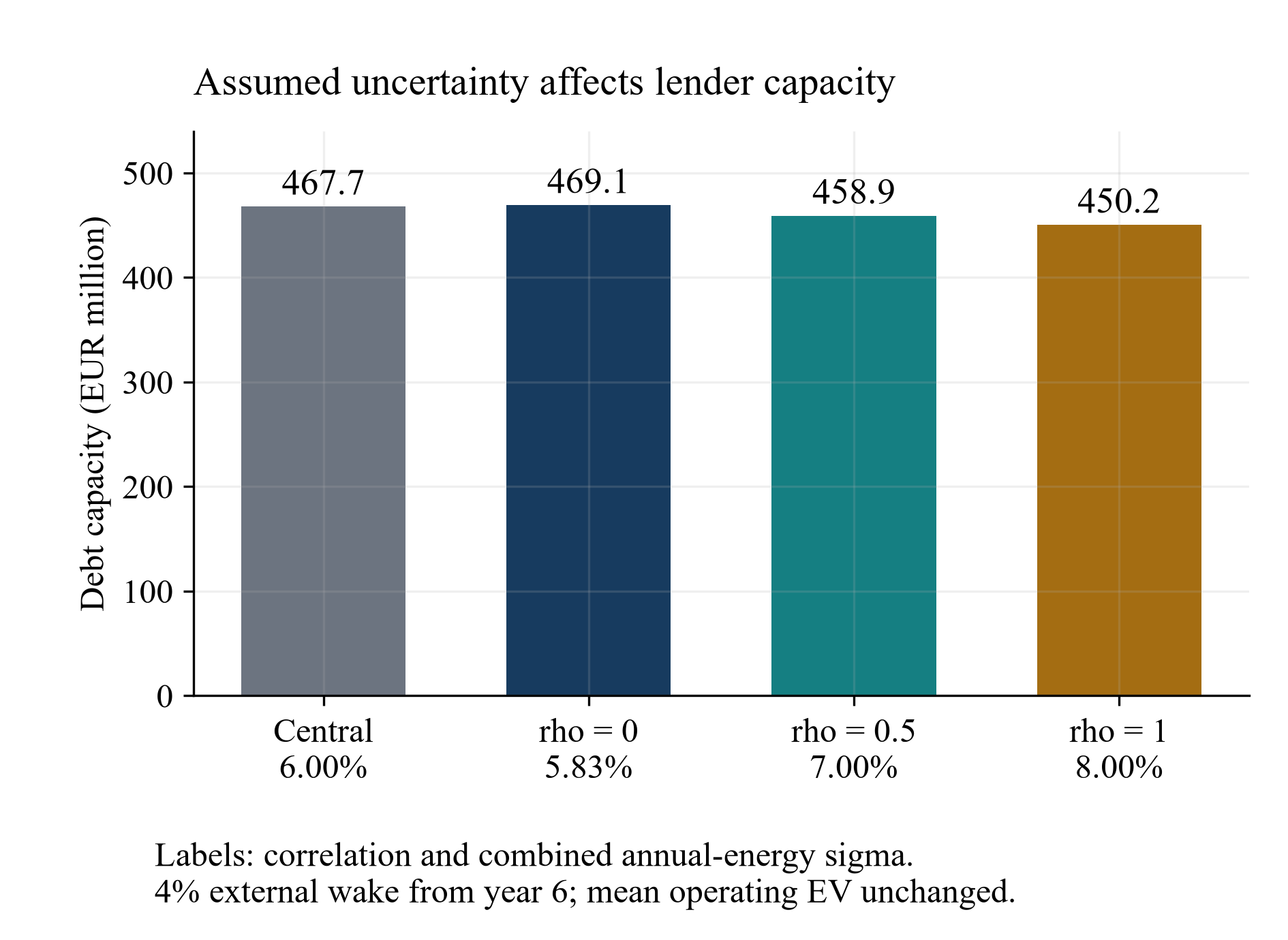
The separate component study assumes resource/other sigma of 5% and wake sigma of 3%. Combined variance equals the sum of their squared sigmas plus twice their product multiplied by the assumed correlation. Zero correlation produces 5.831% combined sigma. Correlations of 0.5 and 1 produce 7% and 8%. The central 6% assumption remains separately identified; 5% and 3% independent components do not combine to exactly 6%.
Table 9. Assumed component correlation and financing capacity.
| Uncertainty convention | Annual sigma | Debt capacity, EURm | Closing equity, EURm |
|---|---|---|---|
| Central input | 6.000% | 467.7 | 502.6 |
| Components, correlation 0 | 5.831% | 469.1 | 501.2 |
| Components, correlation 0.5 | 7.000% | 458.9 | 511.4 |
| Components, correlation 1 | 8.000% | 450.2 | 520.1 |
Entirely hypothetical; 4% external wake from year 6; mean operating EV remains EUR940.3m in every row; component sigmas are 5% and 3%.
Expected generation stays unchanged in this sensitivity, so operating EV stays unchanged. The assumed correlations describe uncertainty dependence, with no assertion about any asset's physical conditions. The positive-correlation cases reduce proxy CFADS and capacity. Figure 4 makes that model channel visible while retaining the central-input comparison.
View figure at full size; scroll horizontally on smaller screens.
Hypothetical correlations between 5% resource/other and 3% wake sigma are separate from the central 6% sigma assumption.
17 Discount-rate sensitivity and the value of further evidence
Hypothetical illustration. Holding the 4% year-6 cash-flow scenario constant, discount rates of 7%, 8% and 9% give operating values of EUR1,013.5 million, EUR940.3 million and EUR875.2 million. Debt capacity remains EUR467.7 million because its separate rate and debt-service inputs are unchanged.
Table 10. Discount-rate sensitivity in the 4% year-6 scenario.
| Operating discount rate | Operating EV | Debt capacity |
|---|---|---|
| 7% | 1,013.5 | 467.7 |
| 8% | 940.3 | 467.7 |
| 9% | 875.2 | 467.7 |
Entirely hypothetical; mean operating cash flows are unchanged; acquisition debt uses its own assumed 5.5% discount rate; amounts EURm.
A measurement sensitivity separately assumes annual sigma falls from 6% to 4%, with unchanged mean energy and lender acceptance. In the 4% year-6 wake case, capacity rises from EUR467.7 million to EUR485.1 million. The EUR17.5 million increase is incremental debt proceeds. Operating EV remains EUR940.3 million. Economic information value requires a specified acquisition decision and defensible probabilities.
For a separate invented decision example, assume a 50/50 prior over zero external wake and 4% external wake from year 6, a bid at their EV midpoint of EUR955.3 million, and an 80%-accurate symmetric measurement signal. The assumed objective maximises expected unlevered NPV with the option to decline. Before information, expected acquisition surplus is zero. A low-wake signal raises the conditional expected surplus to EUR9.0 million; a high-wake signal gives a negative EUR9.0 million surplus. Acquiring only on the low-wake signal gives gross expected value of sample information of EUR4.5 million. An assumed EUR1 million study cost leaves EUR3.5 million. Perfect information would be worth EUR7.5 million under the same invented prior, price and action set.
These decision probabilities, signal accuracy, cost and bid are assumptions, with no real-asset calibration. The example identifies the decision conditions that make information valuable. It supplies no estimate of an actual study's value. The deterministic operating model also omits degradation, merchant prices, additional curtailment, working capital, tax, decommissioning and financing frictions. An asset application requires those inputs and an engineering evidence chain.
An asset-specific model should retain each year's generation, cash flow, debt service and closing balance so that another analyst can reconstruct the result. Its sensitivity schedules should preserve the same timing and units as the agreed purchase-price bridge. Figure 5 shows how the assumed loss and operating discount rate jointly affect finite-life operating value.
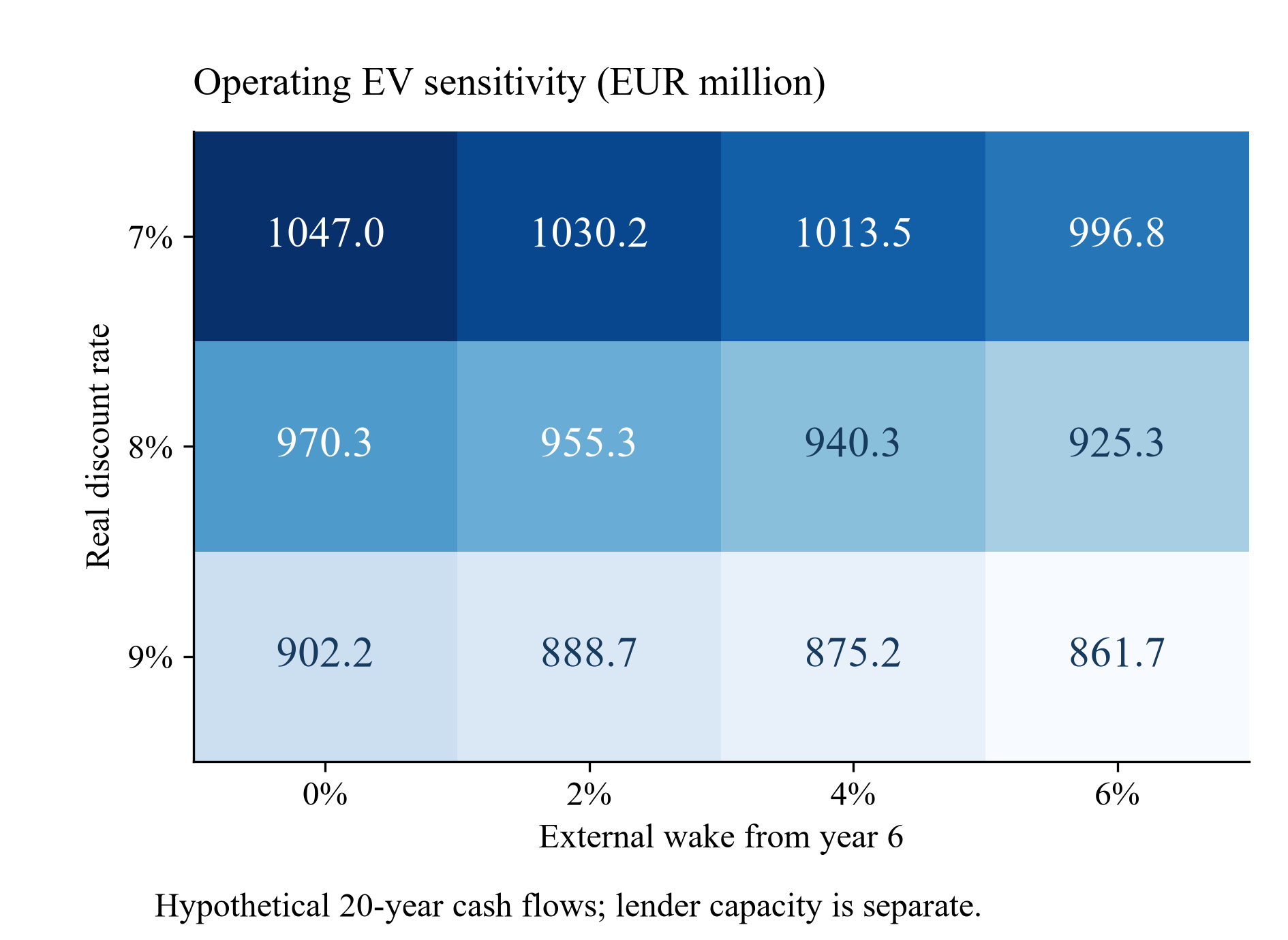
View figure at full size; scroll horizontally on smaller screens.
Hypothetical 20-year pre-tax real cash flows; external wake begins in year 6; zero terminal value.
18 Purchase price and acquisition funding
The investment committee should approve two connected schedules. The first converts the supported operating assumptions into enterprise value and seller equity consideration. The second identifies the funds required to complete the acquisition. Their definitions differ. Enterprise value represents the operating cash flows under the stated valuation convention. Seller equity consideration follows after the agreed existing net debt and other completion adjustments. Acquisition funding identifies the buyer's new debt proceeds, equity contribution, fees and reserves. Keeping these schedules separate makes a wake-related change visible without counting it twice.
The hypothetical model in this paper discounts pre-tax operating cash flow at a specified rate. Its operating value therefore remains independent of the illustrative lender's debt-capacity calculation. If an external wake reduces both operating value and available acquisition debt, the reduction in debt proceeds raises the buyer's equity funding requirement at an unchanged purchase price. It does not create an additional deduction from the same unlevered operating value. A separate financing-cost valuation would need an explicit financing-benefit convention and its own assumptions. It cannot be inserted into the operating bridge as an unexplained discount.
Before final bid, the financial adviser should reconcile the seller model, the buyer model and the financing model at the same valuation date. Differences in inflation, tax, operating period, maintenance capital, decommissioning and discount timing should be resolved before assigning the residual difference to wake modelling. A report that changes several inputs at once can conceal the value attributable to the disputed technical assumption. A reproducible comparison changes one identified set of assumptions and records which other inputs remain fixed.
The purchase agreement also needs a clear debt convention. An assumed repayment of existing project debt, a debt-free acquisition and an acquisition subject to continuing debt generate different completion statements. Existing net debt and new acquisition funding should have separate labels even when the amounts happen to coincide. The transaction team should specify treatment of shareholder loans, accrued interest, restricted cash, break costs, reserves and derivative settlement with the relevant advisers. This paper supplies no asset-specific classification of those items.
Table 11. Separate value and funding schedules
| Schedule | Calculation | Wake-related change | Review boundary |
|---|---|---|---|
| Operating enterprise value | Discounted operating cash flow | Generation and revenue assumptions change | No second deduction for lower acquisition debt |
| Seller equity consideration | Enterprise value less agreed existing net debt and other adjustments | Operating value changes with fixed debt convention | Completion definitions require transaction advice |
| Buyer equity funding | Total uses less new debt and other committed sources | Lower debt proceeds increase the equity contribution at a fixed price | Fees and reserves must enter uses explicitly |
| Financing benefit or cost | Separate, explicitly defined valuation if required | Debt terms may change financing economics | No financing effect included in this paper's operating EV |
Author-proposed transaction definitions; the hypothetical model uses a simplified debt-free operating valuation and an explicit existing-net-debt bridge.
19 Choosing a measurable purchase price mechanism
The author-proposed selection test begins with the question that remains unresolved at signing. A documented input error can support a corrected price before completion. A future study result may support deferred consideration when the study, method, deadline and calculation are agreed. A future neighbouring development may support an event-linked payment when its status can be observed and its value consequence has been modelled. A broad disagreement about future weather needs a range of underwriting cases. Each mechanism requires a fact or event that the parties can identify without reopening every commercial assumption.
For a study-linked adjustment, the parties should specify the permitted study rather than require a future report to state the correct wake loss. The schedule should identify the asset layout, turbine configuration, reference meteorology, neighbouring-project cases, modelling software and comparison period. It should state whether a measurement result changes a model parameter, a central energy estimate or an uncertainty term. A reduction in uncertainty can affect the financing case while leaving mean production unchanged. An agreement that pays on either outcome using the same formula would blur that distinction.
A contingent-payment formula needs an agreed valuation conversion. If the payment is linked to a change in annual net generation, the schedule should define the affected years, revenue convention, avoided variable cost, tax treatment and discount date. Caps and floors define negotiated limits; they provide no evidence about the physical loss. Payment timing changes present value, so a later payment should be compared on the same valuation-date basis. The numerical examples in this paper illustrate that timing mechanism without proposing market-standard caps, survival periods or pricing terms.
An escrow secures a defined payment or claim subject to its governing arrangements. The transaction team must still agree the underlying calculation and release instructions. A funded account cannot resolve an ambiguous measurement test. A holdback raises separate questions about the seller's credit exposure to the buyer. Counsel and the parties should review custody, interest, tax, insolvency, dispute and release provisions against the transaction's governing law. No enforceability or insurance coverage conclusion is made here.
Table 12. Match the unresolved question to a transaction mechanism
| Unresolved question | Possible mechanism | Evidence or calculation required | Principal failure mode |
|---|---|---|---|
| Confirmed input error before completion | Agreed price correction | Versioned rerun with unchanged other assumptions | Changing revenue or discount inputs at the same time |
| Independent study due after signing | Completion condition or deferred payment | Named method, delivery standard and objective acceptance test | An open-ended requirement for a satisfactory report |
| Future neighbouring project status | Event-linked consideration | Official status, layout scenario and timing convention | Treating announcement and construction as identical |
| Disclosed, defined exposure | Escrow or holdback | Claim or payment formula and release instructions | Security without a workable underlying test |
| Seller evidence or disclosure failure | Negotiated warranty or specific protection | Specified statements, causation and remedy | Converting factual disclosure into a weather promise |
Author-proposed selection framework, not observed market terms or legal advice. Counsel must assess drafting and enforceability.
20 Designing post closing measurement
A post-closing test should be designed before the acquisition documents are signed. The parties need to know what observations can answer the disputed question and how long a useful sample is likely to take. Direction, atmospheric stability, season, turbine availability and neighbouring-farm operating status can influence the comparison. The SCADA monitoring research and annual simulation studies reviewed in this paper support attention to those conditions [4][5][9]. They provide no universal minimum measurement period for a contractual payment test.
The protocol should name the measurement boundary. Turbine production, collection-system output and the revenue meter can differ because of electrical losses and other operating effects. Each input needs a timestamp convention, unit, source and quality flag. The parties should preserve raw observations and a separate cleaned dataset so that exclusions remain auditable. A calculation that permanently overwrites raw data prevents later review of whether a filter changed the reported result.
Normalisation should address the specific source of uncertainty under negotiation. A test intended to assess external wakes should record relevant neighbouring turbine operation and compare equivalent wind states where the evidence permits. It should also specify the treatment of turbine downtime, derating, grid instructions, environmental stops and control changes. Assigning every observed production shortfall to an external wake would merge unrelated causes. Where the evidence cannot separate them reliably, the protocol should state how the resulting uncertainty affects the payment decision.
The buyer needs operational discretion for safety, maintenance and legal compliance. A contingent metric can create an incentive to change dispatch or defer work, so permitted actions and recordkeeping should be agreed. The protocol should explain how an upgrade, wake-steering intervention or changed turbine operating mode alters the comparison. Keeping an old model frozen for contractual calculation may be appropriate while a different model informs daily operations. Both versions need clear labels and a reconciliation.
Insufficient data should have a defined outcome. Possible negotiated responses include a limited extension, an alternative independent study, a formula using agreed remaining evidence or a fixed allocation after a long-stop date. The preferred response depends on the asset and the parties' risk allocation. An indefinite measurement obligation can leave consideration unresolved long after asset management has changed. The author-proposed protocol therefore includes a data sufficiency test and a finite decision timetable.
21 Evidence management and independent determination
The technical baseline should contain enough information for a qualified reviewer to reproduce the material outputs. Required records include input datasets, layouts, turbine parameters, model settings, software versions, cleaning rules and output files. Reliance rights, software licensing and confidentiality should be addressed through the adviser and transaction arrangements. Possession of a report alone does not establish a contractual right to rely on its conclusions; this paper makes no statement about a particular engagement's rights.
Every change between the indicative bid and completion should record its reason and its consequences. An updated neighbouring-project layout may change mean energy, the range of cases or both. A revised data-cleaning rule can change apparent availability and the calibration sample. A software update can change the modelling method even where all physical inputs remain identical. The change register should identify whether the technical report, investment model, lender submission and purchase schedule have all received the same update.
An independent expert's remit should identify the question to determine and the boundaries of discretion. For example, the expert may check compliance with an agreed calculation procedure, resolve a stated input dispute or assess whether a measurement sample meets a defined sufficiency standard. A mandate to determine fair value would require broader financial assumptions and professional scope. The parties should distinguish these roles in the appointment and seek advice on the governing determination procedure.
The evidence register should also preserve unsuccessful or excluded cases when they materially informed the decision. Removing an alternative because it produces an inconvenient result undermines the comparison. A defensible register explains why a case was included, rejected or retained as a sensitivity. The source reviews in this paper illustrate the same discipline: a simulation benchmark, a programme objective and a vendor performance statement carry different evidential weight [6][7][12][13].
Table 13. Minimum reproducibility records at signing
| Record | Required contents | Responsible review | Acceptance question |
|---|---|---|---|
| Physical configuration | Site boundary, layout, turbines, controls and adjacent projects | Technical adviser | Can the reviewer reconstruct the modelled configuration? |
| Observation archive | Raw data, units, timestamps, quality flags and exclusions | Technical adviser and operator | Can cleaned data be traced to original observations? |
| Model archive | Version, parameters, scripts, licences and outputs | Independent technical reviewer | Can the material cases be rerun or independently checked? |
| Financial conversion | Revenue, costs, tax, period and discount convention | Financial adviser | Is each technical change priced once? |
| Contract calculation | Trigger, formula, limits, timing and dispute process | Counsel and financial adviser | Can the payment be calculated within the agreed remit? |
| Change register | Old and new inputs, reasons, approvals and affected documents | Deal lead | Do all signing documents use the same approved baseline? |
Author-proposed register for a transaction team; project-specific advisers determine the required deliverables and reliance arrangements.
22 Portfolio acquisitions and refinancing
A portfolio acquisition should begin with site-level analysis because the physical sources of uncertainty differ. One farm may have long operating records and stable neighbouring layouts. Another may have incomplete data, a recently changed control system or exposure to a development that has yet to reach construction. A single portfolio wake percentage can conceal those differences. The financial model should retain the site-level cash-flow calculation before aggregating the transaction value.
Diversification depends on the relevant dependency. Weather exposure across nearby farms, a shared reference dataset, the same modelling method and a common future cluster development can produce related errors. The author-proposed review distinguishes variability across sites from a systematic bias that affects several estimates together. The uncertainty-component example in Section 16 demonstrates the arithmetic consequence of correlation. It does not estimate a real portfolio correlation or a lender's accepted diversification benefit.
Allocation of consideration requires similar care. A portfolio-level cap or basket may simplify negotiation, but the calculation should still identify which site generated a payment. Cross-site netting can expose one party to unrelated operating actions or data gaps elsewhere in the portfolio. Any such netting should be deliberate and documented. Site-level expert outputs may be needed even when the final consideration is settled at portfolio level.
The acquisition evidence can support subsequent asset management and refinancing when it remains current. The owner should update neighbouring-project status, control changes, production reconciliation and major maintenance assumptions. A lender or buyer may require its own scope, reliance rights and technical case. The availability of an archived acquisition report does not establish acceptance for a later financing. Its practical value is the ability to explain the original decision and identify which assumptions have changed [14].
23 Implementation responsibilities and decision thresholds
The proposed workplan assigns each question to an owner and a decision date. The technical adviser reconstructs generation and uncertainty. The financial adviser converts the cases into value and acquisition funding. Counsel specifies the price mechanism and evidence obligations. The deal lead reconciles those workstreams before bid, signing and completion. The investment committee approves the remaining assumptions and the risk retained by the buyer. These are proposed responsibilities; a transaction engagement should define the actual appointments.
Escalation should depend on materiality and evidence quality together. A large value sensitivity supported by limited observations merits early attention. A small sensitivity can still matter if it invalidates a contractual statement or a financing condition. The team should record the maximum affordable diligence cost, the decision it could change and the timetable within which useful evidence can arrive. A measurement campaign that completes after the final decision needs a contingent mechanism or a different purpose.
The decision pack should identify the supported central case, the selected downside cases and unresolved limitations. It should show how the proposed bid changes when the external wake starts earlier, loss increases or the required return changes. The funding schedule should show the buyer's equity commitment at the proposed price under the financing cases. If the required equity exceeds the approved contribution, the team needs an agreed response before signing. That response might involve price, structure, further committed funding or a decision not to proceed.
Table 14. Decisions and work products across the acquisition
| Decision stage | Required work product | Decision owner | Unresolved item to record |
|---|---|---|---|
| Indicative bid | Initial yield reconciliation and bounded value range | Investment committee | Missing operating data and external-project status |
| Final bid | Reproducible technical cases and separate value/funding schedules | Investment committee with advisers | Sensitivities that could change price or equity commitment |
| Signing | Frozen baseline and agreed calculation or risk allocation | Transaction principals and counsel | Evidence deliverables and objective acceptance conditions |
| Completion | Updated status and confirmed sources and uses | Deal lead and funding parties | Changes since signing and remaining payment obligations |
| Post closing | Measurement outcome and operating-model reconciliation | Asset manager and appointed reviewer | Data sufficiency, control changes and unresolved determination |
Author-proposed sequence; timing and responsibilities depend on the actual process and available evidence.
24 Limitations and conclusion
This paper combines published technical evidence with an author-proposed acquisition framework and an explicitly hypothetical financial model. The reviewed studies use different locations, layouts, atmospheric conditions, reference datasets and validation methods. Their results cannot be transferred into the annual production estimate of an unassessed asset. Model disagreement identifies a diligence question. It does not, by itself, identify the correct loss, a probability distribution or an appropriate price concession.
The illustrative model omits taxes, inflation, hourly merchant pricing, degradation, reserve funding, fees, construction costs and decommissioning liabilities. Its finite operating period and zero terminal value are assumptions. Its P90 calculation is an uncalibrated normal approximation. The financing calculation is a selected coverage constraint rather than an observed credit offer. These simplifications allow the reader to reproduce the separate operating-value and funding effects. A transaction requires a substantially more detailed model and asset-specific technical, financial, legal and tax review.
The useful acquisition discipline is to connect each material adjustment to a defined physical assumption, evidence source and cash-flow consequence. Expected wake loss changes central production. Uncertainty changes the confidence attached to that estimate and can affect a selected financing case. External development timing changes the years exposed to a loss. Those mechanisms should remain visible through the investment model and the acquisition documents.
A buyer can use this framework to identify the evidence required before final bid, calculate the range supported by its assumptions and specify a measurable allocation of the remaining risk. The resulting price and equity commitment remain transaction decisions. Their defensibility depends on the quality of the asset-specific evidence, the chosen valuation convention and the ability to reproduce the calculation at the relevant decision date.
References
- International Electrotechnical Commission. IEC 61400-15-1:2025: Wind energy generation systems; Part 15-1: Site suitability input conditions for wind power plants. 14 March 2025. Public publisher description; full paid standard not accessed. https://webstore.iec.ch/en/publication/29169 Accessed 11 October 2026.
- Fuchs, R., et al. Assessment of Offshore Wind Energy Opportunities and Challenges in the U.S. Gulf of Mexico. NREL/TP-5000-88195. December 2023. https://docs.nlr.gov/docs/fy24osti/88195.pdf Accessed 11 October 2026.
- Cooperman, A., Duffy, P., Hall, M., Lozon, E., Shields, M., and Musial, W. Assessment of Offshore Wind Energy Leasing Areas for Humboldt and Morro Bay Wind Energy Areas, California. NREL/TP-5000-82341. April 2022. https://docs.nlr.gov/docs/fy22osti/82341.pdf Accessed 11 October 2026.
- Porchetta, S., Howland, M. F., Lejeune, M., Borgers, R., Buckingham, S., and Munters, W. Annual wake impacts in and between wind farm clusters; Part 2: Comparison of WRF and fast-running engineering wake models. Wind Energy Science 11, 3295-3319. 7 September 2026. https://wes.copernicus.org/articles/11/3295/2026/ Accessed 11 October 2026.
- Rosencrans, D., Lundquist, J. K., Optis, M., Rybchuk, A., Bodini, N., and Rossol, M. Seasonal variability of wake impacts on US mid-Atlantic offshore wind plant power production. Wind Energy Science 9, 555-583. 14 March 2024. https://wes.copernicus.org/articles/9/555/2024/ Accessed 11 October 2026.
- Aerts, F., Devesse, K., and Meyers, J. Bayesian uncertainty quantification of engineering models for wind farm-atmosphere interaction. Wind Energy Science 11, 1205-1225. 14 April 2026. https://wes.copernicus.org/articles/11/1205/2026/ Accessed 11 October 2026.
- Bodini, N., et al. The AWAKEN wind farm benchmark; Part 2: Modeling results. Wind Energy Science 11, 3107-3135. 27 August 2026. https://wes.copernicus.org/articles/11/3107/2026/ Accessed 11 October 2026.
- Elizalde, A., Akhtar, N., Geyer, B., and Schrum, C. Uncertainty in North Sea offshore wind power: contributions of reanalysis forcing, turbine type, and wake parameterization. Wind Energy Science 11, 1077-1095. 1 April 2026. https://wes.copernicus.org/articles/11/1077/2026/ Accessed 11 October 2026.
- Mittelmeier, N., Blodau, T., and Kühn, M. Monitoring offshore wind farm power performance with SCADA data and an advanced wake model. Wind Energy Science 2, 175-187. 28 March 2017. https://wes.copernicus.org/articles/2/175/2017/ Accessed 11 October 2026.
- Cameron, L., Clerc, A., Feeney, S., and Stuart, P. Remote Wind Measurements Offshore Using Scanning LiDAR Systems. RES report for Carbon Trust Offshore Wind Accelerator. Public final report; publication date not stated in inspected file. https://www.carbontrust.com/sites/default/files/documents/resource/public/owa-scanning-lidar-final-report-public-version.pdf Accessed 11 October 2026.
- Carbon Trust. OWA GloBE measurement campaign extended to bolster data and analysis on Global Blockage Effect in offshore wind farms. 31 March 2022. https://www.carbontrust.com/en-eu/news-and-insights/news/owa-globe-measurement-campaign-extended-to-bolster-data-and-analysis-on-global-blockage-effect-in-offshore-wind-farms Accessed 11 October 2026.
- Carbon Trust. Yield and performance; Offshore Wind Accelerator. Undated programme page. https://www.carbontrust.com/en-eu/our-work-and-impact/impact-stories/offshore-wind-accelerator-owa/yield-and-performance Accessed 11 October 2026.
- DNV. Offshore turbine interaction modelling using CFD.ML. Undated public landing page; implementation date stated as 1 June 2026. Full form-gated whitepaper not accessed. https://www.dnv.com/publications/offshore-turbine-interaction-modelling-using-cfd.ml Accessed 11 October 2026.
- DNV. Operational energy assessment of renewables. Undated service description. https://www.dnv.com/services/operational-energy-assessment-of-renewables-3961/ Accessed 11 October 2026.
About the Author
Chennakeshav (CK) is a corporate finance and investment banking executive with 25+ years of global experience in deal origination, structuring and execution across M&A, growth capital and corporate strategy. He has led value-creation mandates for founders, corporates and funds — bridging the boardroom view to hands-on execution and close.
His career spans Morgan Stanley, HSBC, Lloyds Banking Group, EWEC, ADQ portfolio companies and Emirates Growth Fund, across TMT, real estate, fintech, deeptech, cleantech, infrastructure and energy. He has partnered with C-suite leaders, private equity and venture funds, sovereign wealth funds and family offices to finance complex fund raises and scale-up ventures, and has led M&A due diligence, post-merger integration and business-transformation initiatives to create value.
At Matchpoint Partners he is Managing Partner, leading the firm's corporate finance, M&A and capital-raising practice. He holds an MBA from London Business School, an engineering degree from VTU and a Master of Laws (LLM, in progress) from UCL London.
An active start-up mentor, CK mentors at Techstars, DIFC FinTech Hive, Startup Grind, Founder Institute and IN5, serves as Entrepreneur Mentor in Residence (EMiR) at London Business School, and judges the Entrepreneurship World Cup.
https://www.linkedin.com/in/ckadya/
https://www.matchpoint-partners.com/team/ck-adya.html
Disclaimer
This paper is part of a continuing series on the structure of private and alternative markets. The views expressed are the author's own. The paper is for information only, describes market structure in general terms, and does not constitute investment, legal, tax or regulatory advice or a recommendation in respect of any security, vehicle or counterparty.
