

The constrained capital-stack decision
Audience and Decision Perimeter
Primary audiences
It identifies as infrastructure and digital-infrastructure investors providing infrastructure debt and equity. Their decision interests overlap while their duties remain distinct.
A sponsor needs a financeable path from development rights and power access to phased construction and contracted capacity. Its model must expose the timing and source of every cash requirement, the conditions attached to each facility, the liquidity effect of delay, and the point at which committed demand supports additional investment. An investor needs to understand downside protection, governance, completion exposure, power and offtake concentration, refinancing risk, residual value and whether the proposed financing retains resilience under adverse scenarios.
Decision rights
Companion topics
It would test hardware eligibility, depreciation assumptions, refresh cycles, remarketing channels, advance rates and offtake support. It would test land control, connection deposits, design, permits and long-lead orders before a construction lender is prepared to fund.
Advice perimeter
An optimisation output is a model result. It is not a financing offer, valuation, legal interpretation, technical certification, grid commitment, tax opinion, accounting judgement or investment recommendation. Any transaction use requires approved source data, professional review, counterparty engagement and executed documents.
Why The Capital Stack Is A Constrained Optimisation Problem
Connected decisions
A capital stack becomes an optimisation problem when several feasible structures exist and management wants to select among them using a declared objective. Typical objectives include minimising expected all-in funding cost, minimising expected equity requirement, maximising risk-adjusted project value, maximising liquidity headroom, minimising refinancing exposure or finding a robust compromise across several measures.
The decision set is combinatorial. A tranche can be selected or rejected. A phase can start in one of several periods. A power contract can cover a selected share of load. An equipment order can be accelerated or deferred. A reserve can be funded from equity or facility proceeds if documents permit. These discrete choices interact with continuous amounts such as debt size, equity contribution, power volume and cash reserve.
Constraint families
Mathematical class
Many core relationships can be written as a mixed-integer linear programme, or MILP. Binary variables represent selection and sequencing decisions; continuous variables represent money, capacity and energy; and linear constraints enforce balances, timing and thresholds. Quadratic terms arise when the objective includes variance, pairwise concentration, nonlinear penalty interactions or a direct QUBO encoding. Some relationships are nonlinear or discontinuous and may require piecewise-linear approximations, mixed-integer nonlinear programming, decomposition or simulation outside the optimiser.
The choice of mathematical form matters. A QUBO is not automatically the best representation for the classical baseline. A constrained model may be more compact and more interpretable. Fair benchmarking gives each solver the formulation that best fits its architecture while preserving equivalent information and an equivalent decision problem [28-31].
Feasibility before optimality
Every candidate solution must satisfy hard legal, contractual, technical and policy constraints before its objective value is considered. A cheaper plan that misses an energisation gate, violates a funding-eligibility rule or exhausts minimum liquidity is infeasible. Penalty formulations used for QUBO or Ising models must be calibrated and independently tested so that apparent objective improvement cannot be purchased through an unrecognised constraint breach.
Figure 2. Data-centre capital-stack timeline and dependency graph
Source: Matchpoint framework; energy and infrastructure context [1-10,17].
Canonical Decision Model
Model objects
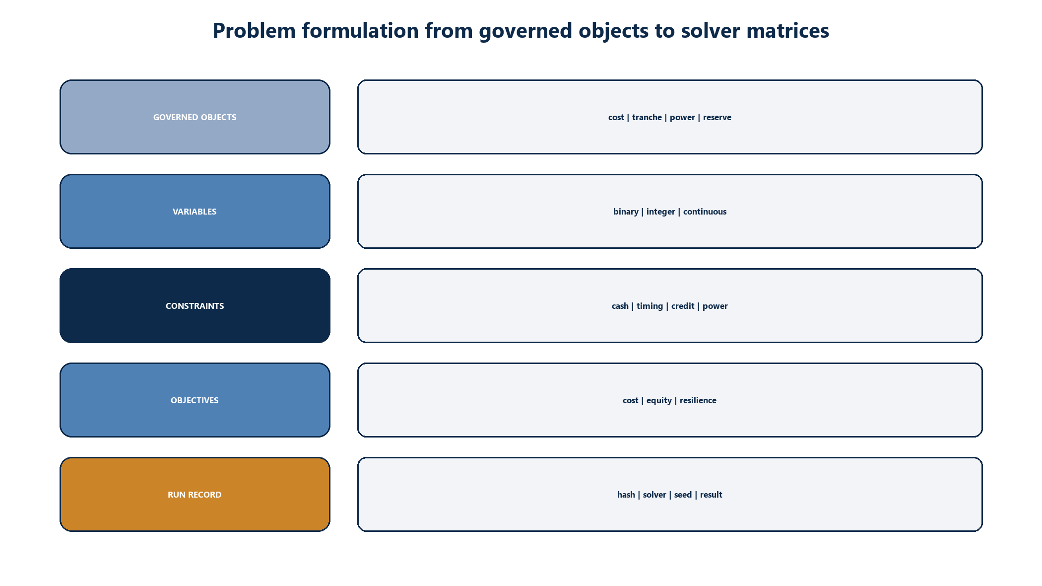
The proposed canonical model stores each consequential assumption as a versioned object with source, owner, as-of date, unit, scenario, confidence or approval state and refresh trigger. A solver-ready matrix is derived from these objects. It is not the system of record.
Time and currency
Time is represented in explicit periods, normally months for development and quarterly or annual aggregation for longer-term credit analysis. Each amount retains native currency, approved foreign-exchange source, conversion time and hedge treatment. Nominal and real values are never mixed silently. Interest conventions, day counts, compounding and fees remain explicit.
Source hierarchy
Executed contracts, lender-approved definitions, utility confirmations, board-approved budgets and validated technical schedules take precedence over marketing material, indicative terms and management estimates. Management estimates may be used in scenarios when labelled and approved. Vendor roadmaps remain vendor-supplied evidence and cannot be treated as delivered capability.
Model lineage
Every coefficient in the optimisation instance links to the approved model object from which it was derived. Transformations retain formula version, unit conversion and rounding. The system stores both the business-readable representation and the solver-ready form, enabling reviewers to trace a surprising output to the underlying term or assumption.
Figure 3. Problem formulation from governed objects to solver-ready matrices
Source: Matchpoint optimisation framework; modelling context [18-27,36-45,52].
Objective Function And Trade-Offs
Single-objective formulation
A simple formulation minimises the present value of funding cost and expected penalties:
minimise funding cost + commitment fees + hedging cost + reserve carry + expected delay cost + refinancing penalty + concentration penalty
The components must use approved definitions. Expected values require an approved scenario probability. When probabilities are unavailable, the model should report separate scenarios or robust worst-case measures instead of inventing a probability distribution.
Multi-objective formulation
Sponsors and investors rarely have one objective. A weighted formulation may combine cost, equity requirement, liquidity headroom and resilience. Weights are governance decisions, not solver facts. The preferred approach is to produce a Pareto frontier or a set of constrained alternatives:
minimum cost subject to a required liquidity floor;
minimum equity subject to leverage and coverage limits;
maximum resilience subject to an approved cost cap;
minimum refinancing exposure subject to a target return;
minimum power concentration subject to budget and schedule constraints.
Lexicographic priority
Hard feasibility comes first. The next priority may be completion and liquidity resilience, followed by cost and return. A lexicographic solve preserves that order. It avoids the governance problem created when a small reduction in price mathematically offsets a material reduction in resilience because of an arbitrary weight.
Risk measures
The model can use scenario loss, maximum shortfall, conditional value at risk or a robust uncertainty set. Each method has data and governance requirements. Historical distributions from unrelated markets do not become project probabilities without justification. Scenario design should separate observed inputs, contractual cases, management estimates and deliberately severe stresses.
Tie-breakers
Two solutions can have the same reported objective within tolerance while differing in complexity. The model should use declared tie-breakers such as fewer facilities, fewer intercreditor dependencies, longer committed availability, higher liquidity, lower refinancing concentration or greater source diversity. The rationale remains visible to the investment or credit committee.
| Decision layer | Optimisation object | Retained authority |
|---|---|---|
| Capital structure | Tranche selection, sizing, pricing, tenor and draw order | Sponsor, investment committee and financing counterparties |
| Construction | Phase starts, equipment orders, contingency and completion gates | Sponsor, technical adviser and contractors |
| Power | Interconnection, PPA, grid, onsite generation, storage and flexibility | Sponsor, utility, offtaker and relevant authorities |
| Credit | DSCR, leverage, reserve, covenant and distribution tests | Lenders, credit committee and finance documents |
| Quantum challenger | Candidate solution or sample distribution | Model owner and independent validation; no transaction authority |
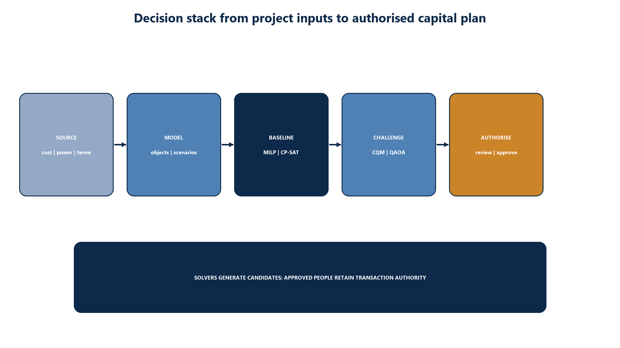
Instruments, draw schedules, power and uncertainty
Capital-Instrument Variables And Constraints
Instrument library
The instrument library may include sponsor equity, preferred equity, shareholder loans, senior construction debt, delayed-draw term debt, bridge facilities, mezzanine or subordinated debt, equipment finance, vendor finance, working-capital facilities, letters of credit, hedging lines, project bonds, sukuk and asset-level or portfolio-level refinancing. Availability depends on jurisdiction, project facts and market engagement.
Selection and sizing
For each instrument k, a binary variable y-k records whether it is selected. A continuous variable d-k records commitment or drawn amount. Linking constraints enforce 0 <= d-k <= y-k x approved-limit-k. Additional constraints represent minimum ticket, currency, cost eligibility, tenor, amortisation, collateral and cross-default relationships.
Draw order
Draw order can be contractual, economic or both. A senior facility may require a minimum equity contribution before first draw. A bridge may be repaid from construction debt after specified conditions. Equipment finance may fund only accepted hardware. The optimiser enforces each rule by period and cost category.
Fees and all-in cost
All-in funding cost includes margins, base rates, original issue discount, arrangement fees, commitment fees, undrawn fees, agency costs, hedging, legal and diligence costs where approved, reserve carry and refinancing assumptions. Taxes and accounting treatment require specialist confirmation. Indicative market terms require support from current transaction correspondence.
Intercreditor and structural constraints
Structural complexity creates constraints that may not appear in a simple weighted average cost of capital. These include collateral sharing, payment blockage, cure rights, cash sweeps, permitted debt, guarantor coverage, account control, transfer restrictions and consent requirements. A structure that cannot be documented on the assumed timetable is not a valid low-cost solution.
Draw-Schedule Optimisation
Monthly cash balance
For every period, opening cash plus permitted funding plus operating receipts equals eligible uses, debt service, reserve movements and closing cash. The minimum cash balance and designated reserves remain separate. A facility cannot fund a use before the use becomes eligible or after its availability expires.
Construction dependencies
The construction schedule is represented as a directed dependency graph. Land control, design, permits, grid studies, interconnection deposits, substation work, long-lead electrical equipment, shell construction, mechanical and electrical completion, commissioning and tenant acceptance may each gate later activities. The model must not compress professional schedules without a validated alternative programme.
Conditions precedent
Each draw gate has evidence, owner and status. The model may test a dated assumption that a condition becomes satisfied. It cannot mark a legal or technical condition satisfied. For transaction use, the current conditions tracker controls availability.
Interest during construction
Interest during construction depends on the timing of debt draws, capitalisation rules and rates. The financing need and financing cost are therefore recursive. A robust formulation may iterate or include linearised balances. The exact implementation must reconcile to the approved financial model.
Delay and liquidity
Delay changes interest, fees, contingency use, reserve duration, offtake commencement and refinancing. The model evaluates explicit delay cases. It should identify the first period and constraint that cause infeasibility, enabling management to distinguish a pricing problem from a liquidity or timing problem.
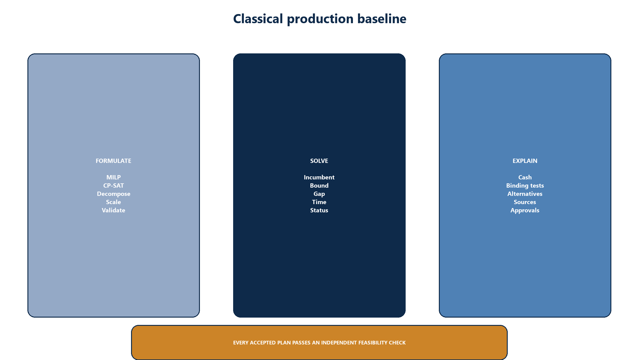
Figure 4. Classical optimisation baseline and audit trail
Source: Matchpoint framework; classical solver guidance [36-40,49-51].
Power-Contract Portfolio
Power as a financing dependency
IEA and DOE sources describe electricity supply, grid connection and equipment availability as binding data-centre constraints [1-6]. A capital plan that assumes unavailable or uncontracted power is not financeable. The model therefore represents power as a dated portfolio of enforceable or explicitly contingent sources.
Source types
Potential sources include grid supply, utility tariff arrangements, physical or financial PPAs, onsite generation, batteries, backup generation and demand flexibility. Each source has capacity, energy, shape, availability, price, tenor, credit, emissions attributes, development risk and legal constraints. The model does not treat different products as economically identical megawatts.
Contract-selection variables
Binary variables select contracts and options. Continuous variables allocate demand by source and period. Constraints enforce contracted capacity, energy balance, ramping, outage or derating assumptions, minimum purchase, maximum volume, start date, tenor, settlement and concentration. Approved engineering studies define technical feasibility.
Shape and coincidence
Annual energy is insufficient for a high-load facility. The model must represent peak demand, ramp, maintenance, cooling load, utilisation and temporal coincidence between supply and load at a resolution supported by evidence. Coarse optimisation may screen strategies; detailed dispatch and grid analysis remain separate specialist work.
Financing interaction
Power choices affect capex, opex, credit support, deposits, letters of credit, completion date, operating risk and lender diligence. A longer PPA may support price certainty while adding termination exposure. Onsite assets may add construction and fuel risk. Flexibility may improve grid integration where technically and contractually permitted. Each effect enters through explicit model objects.
Uncertainty, Scenarios And Robustness
Scenario register
The scenario register separates base assumptions from stresses. Examples include delayed interconnection, equipment-price change, tenant ramp delay, lower utilisation, higher base rates, refinancing margin widening, construction overrun, exchange-rate movement, power-price change and a failed funding source. Each scenario states its source, owner, approval status and affected variables.
Stochastic formulation
A two-stage formulation chooses commitments before uncertainty and draws or operating actions after a scenario is realised. This can model the value of committed liquidity or flexible contracts. Scenario probabilities must be approved. If probabilities are management estimates, the full output is labelled accordingly.
Robust formulation
Robust optimisation seeks a plan that remains feasible across an approved uncertainty set. The uncertainty set may bound cost, delay, rate and demand changes. Wider sets improve stated resilience while usually increasing cost. Management chooses the set; the solver exposes the trade-off.
Stress and reverse stress
Stress testing asks whether the plan survives a defined shock. Reverse stress testing asks which combination of changes first breaches liquidity, coverage, leverage or completion. The latter can reveal hidden dependence on one facility, one power date or one tenant ramp.
Correlation
Power delay, construction delay, capex escalation and tenant commencement can be correlated. Treating them as independent may understate tail exposure. Correlation assumptions require evidence or explicit management approval. The model should provide correlated scenario bundles rather than false precision.
| Object | Minimum fields | Control purpose |
|---|---|---|
| Project phase | Site, building, MW, start, completion and dependency | Defines construction units |
| Cost item | Cost code, phase, amount, currency, timing and eligibility | Defines uses and facility access |
| Capital instrument | Type, commitment, price, tenor, amortisation and conditions | Defines funding choices |
| Draw gate | Instrument, date, evidence, approver and status | Prevents premature availability |
| Power source | Grid, PPA, generation or storage; volume, shape, term and price | Defines supply portfolio |
| Offtake contract | Customer, capacity, term, ramp, credit and termination | Defines revenue support |
| Reserve | Purpose, base, amount, release test and account | Protects liquidity and credit |
| Scenario | Named changes, probability if approved, owner and status | Separates cases from facts |
| Solver run | Model hash, solver, version, parameters, seed, time and result | Supports reproducibility |
Classical baseline and quantum challengers
Classical Production Baseline
Baseline requirement
Quantum evaluation begins after a well-engineered classical baseline exists. Google OR-Tools documents MIP, CP-SAT, branch-and-bound and SAT-based approaches; COIN-OR documents the CBC branch-and-cut solver [36-40]. These tools demonstrate that the relevant classical method depends on model structure. Commercial solvers may also be included under approved licences.
Formulation variants
The baseline suite should include:
a direct MILP for continuous amounts, binary choices and linear constraints;
CP-SAT for predominantly Boolean or integer scheduling and logical structure;
decomposition where master capital choices and subproblem schedules separate naturally;
scenario decomposition for many uncertainty cases;
local search or other heuristics for rapid incumbent generation;
deterministic rules for calculations that do not require optimisation.
Solver evidence
For exact or bound-producing solvers, the run record stores incumbent objective, best bound, optimality gap, feasibility tolerance, elapsed time, node count and termination reason. For heuristics, it stores solution quality, constraint residuals, repeated-run distribution and time-to-target. A result labelled optimal must use the solver's precise status and approved tolerances.
Numerical controls
Scaling and numerical precision matter. OR-Tools guidance notes that floating-point tolerances influence feasibility and optimality claims [39]. Money, capacity and energy units should avoid extreme coefficient ranges. Big-M constants require documented upper bounds. Penalties require sensitivity testing. Every accepted solution is rechecked by an independent deterministic validator.
Production output
The production baseline produces a business-readable plan, sources-and-uses table, draw schedule, covenant and reserve tests, binding constraints, alternative solutions, scenario results, source lineage and approval state. The solver file alone is insufficient.
Quantum Annealing And D-Wave Cqm
Quadratic models
D-Wave's Ocean documentation describes Ising models, QUBO, binary quadratic models and constrained quadratic models [18-22]. A QUBO expresses a binary objective in linear and pairwise terms. Hard constraints are commonly converted into penalties when using an unconstrained representation. D-Wave's CQM abstraction supports binary, integer and real variables with linear and quadratic objectives and constraints [18-20]. These are vendor-supplied descriptions of supported software interfaces.
Annealing workflow
A direct quantum-annealing workflow prepares an Ising or QUBO problem, embeds its logical graph onto the QPU topology, samples many anneals, unembeds the results and validates feasibility. D-Wave documentation explains that minor embedding can represent one logical variable by a chain of physical qubits and that broken chains can occur [21-24]. Embedding overhead and chain-strength selection therefore belong inside the measured compute and quality boundary.
Hybrid CQM workflow
The Leap hybrid CQM solver accepts a constrained model and uses a quantum-classical service [19-20]. The user does not control every internal allocation between classical and quantum components. Any benchmark report must identify the product, version, stated properties, submission size, service time and returned metadata. A favourable hybrid result establishes performance of that delivered hybrid service on the tested instances. It does not isolate QPU advantage.
Capital-stack mapping
Capital-instrument selection, phase activation and contract selection map naturally to binary variables. Amounts, MW and cash balances may remain continuous in a CQM, or they may be discretised into binary encodings for QUBO. Discretisation adds variables and approximation error. Equality constraints, path dependencies and risk measures add couplings. Dense couplings increase direct embedding burden.
Penalty calibration
For QUBO, a hard constraint becomes a penalty. A penalty that is too small can make an infeasible solution look attractive. A penalty that is too large can compress useful objective differences or exceed practical coefficient precision. The benchmark must report penalty derivation, coefficient scaling, feasibility rate and sensitivity. Independent validation rejects every infeasible sample.
Claim boundary
This paper does not verify that D-Wave quantum annealing outperforms a classical solver on a data-centre capital-stack instance. D-Wave documentation establishes available representations and workflows. Peer-reviewed research reports problem-specific quantum-annealing results, including both favourable scaling evidence and limitations [32-35].
Figure 5. Quantum-annealing and hybrid CQM evaluation pipeline Source: Matchpoint evaluation framework; D-Wave documentation and peer-reviewed research [18-24,28-35].
Qaoa And Ibm Qiskit
Algorithm role
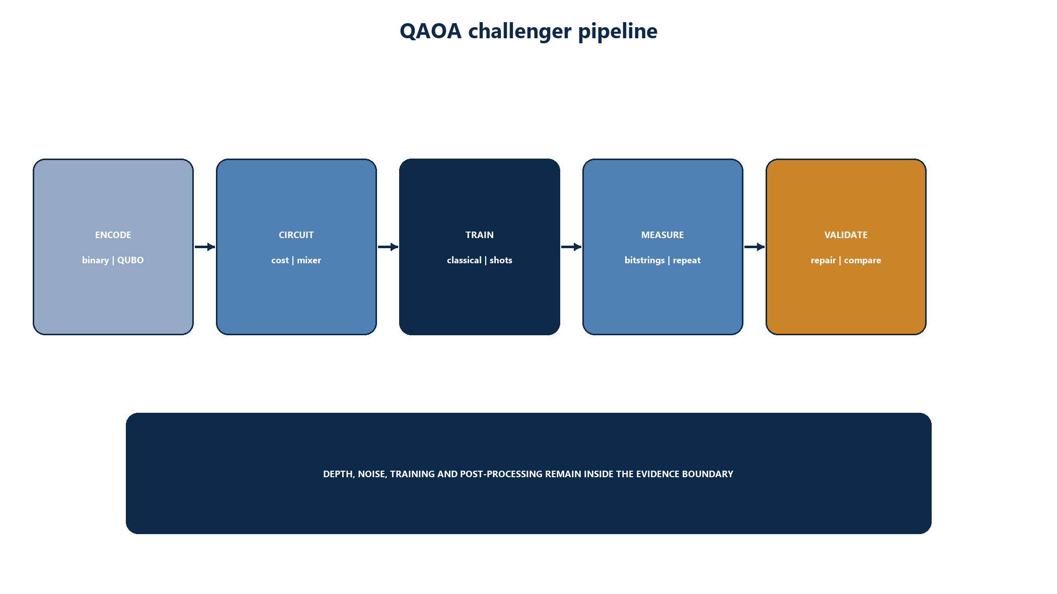
QAOA is a hybrid variational algorithm for combinatorial optimisation. It alternates parameterised cost and mixing operations, measures candidate bitstrings and uses a classical optimiser to update circuit parameters [25-27,41-44]. The algorithm is approximate; performance depends on problem encoding, circuit depth, parameter training, hardware noise, shot budget and classical post-processing.
QUBO and Ising mapping
The capital-stack instance must first be reduced to binary variables and a cost Hamiltonian. Continuous debt or power quantities require discretisation or decomposition. Constraints require a feasible-subspace mixer or penalties. The number of logical variables can grow with the number of instruments, periods, scenarios and precision bits. Mapping the resulting interactions to hardware connectivity adds gates and depth.
Qiskit workflow
IBM Quantum and Qiskit documentation provide tutorials for constructing QUBO problems, transpiling QAOA circuits and executing hybrid quantum-classical workflows [25-27]. Current Qiskit community materials also state the support status of specific optimisation packages and direct users to newer mapping components [27]. The implementation must pin versions and archive source, environment and transpilation outputs.
Warm starts
A classical relaxation or incumbent can initialise a quantum challenger. Qiskit documentation includes a warm-start QAOA workflow [26]. Peer-reviewed work also studies adaptive-bias and warm-start variants [45]. In a fair benchmark, the classical effort used to create the warm start belongs inside total resource accounting and is also available to a comparable classical improvement method.
Evidence from the literature
Peer-reviewed studies provide mixed, problem-specific evidence. PRX and Physical Review papers describe QAOA mechanisms, possible scaling windows and limitations [41-45]. A 2025 Physical Review Research paper concludes that QAOA's ability to deliver quantum advantage on the tested higher-order constraint-satisfaction problems remained unclear and found a mean-field classical method at least as strong on average in the examined regime [43]. A 2024 PRX Quantum paper reports a favourable scaling result for a specific random 8-SAT setting beyond a stated depth relative to the classical solver it tested [44]. Neither result is evidence for a finance problem.
Current hardware roadmap
IBM's 2026 quantum roadmap sets goals for quantum advantage, deeper circuits and later fault-tolerant systems [46-48]. IBM explicitly states that roadmap information represents current intent and may change [46].
Figure 6. QAOA challenger from QUBO encoding to validated candidate plan
Source: Matchpoint evaluation framework; IBM, Qiskit and peer-reviewed research [25-31,41-48].
D-Wave And Ibm Landscape
Architecture comparison
What can be tested now
Small and medium research instances can be generated from a controlled capital-stack model. Classical exact or bound-producing solvers establish reference results where tractable. D-Wave CQM can test the constrained service representation. Direct annealing can test selected binary subproblems. IBM simulators can test QAOA formulation and parameter behaviour before approved hardware runs. Current hardware tests remain experiments; transaction decisions continue to use validated classical or professionally reviewed plans.
What should wait
Large fault-tolerant algorithm claims, deep circuit requirements and hardware capabilities outside delivered service should remain in a research backlog. A sponsor should not make a financing commitment, power contract or construction schedule depend on a vendor roadmap milestone.
Procurement neutrality
The benchmark specification should remain vendor-neutral. It defines inputs, outputs, metrics, compute boundary and acceptance tests. A supplier may propose annealing, gate-model, tensor-network, GPU, CPU, hybrid or specialist classical methods. The best validated solution within the approved service, risk and cost envelope advances.
Encoding And Decomposition
Decompose by decision horizon
The full data-centre model may be too large or too dense for a single challenger formulation. A controlled decomposition can separate strategic facility and power-contract selection from detailed monthly draws, dispatch and covenant calculation. The master problem selects a structure. Deterministic subproblems validate schedule, cash and technical feasibility.
Decompose by asset or phase
Campus phases may be modelled separately with shared constraints for grid capacity, common infrastructure, portfolio facilities and tenant concentration. Coordination variables allocate scarce capacity and liquidity. Any decomposition must converge to a globally consistent plan or state its approximation.
Binary precision
A continuous amount represented with binary bits requires a range and increment. Finer increments increase logical variables. Coarser increments create rounding and may falsely remove feasible structures. The model records precision by variable and reoptimises or validates the rounded result in the original continuous model.
Constraint-preserving design
Some constraints can be encoded through variable construction or mixers rather than penalties. Others are easier to validate after sampling. The selected method must disclose which constraints are guaranteed by representation, encouraged by penalty or tested after solution.
Repair
A classical repair heuristic may convert a near-feasible quantum sample into a feasible plan. The repair algorithm, time and objective change are part of the challenger. The benchmark reports raw feasibility and repaired feasibility separately. A repaired result cannot be presented as the direct quantum output.
Classical-Versus-Quantum Benchmark
Evidence state
The benchmark in this section is a design specification. All instance sizes, target times and acceptance thresholds require approval before execution.
Benchmark question
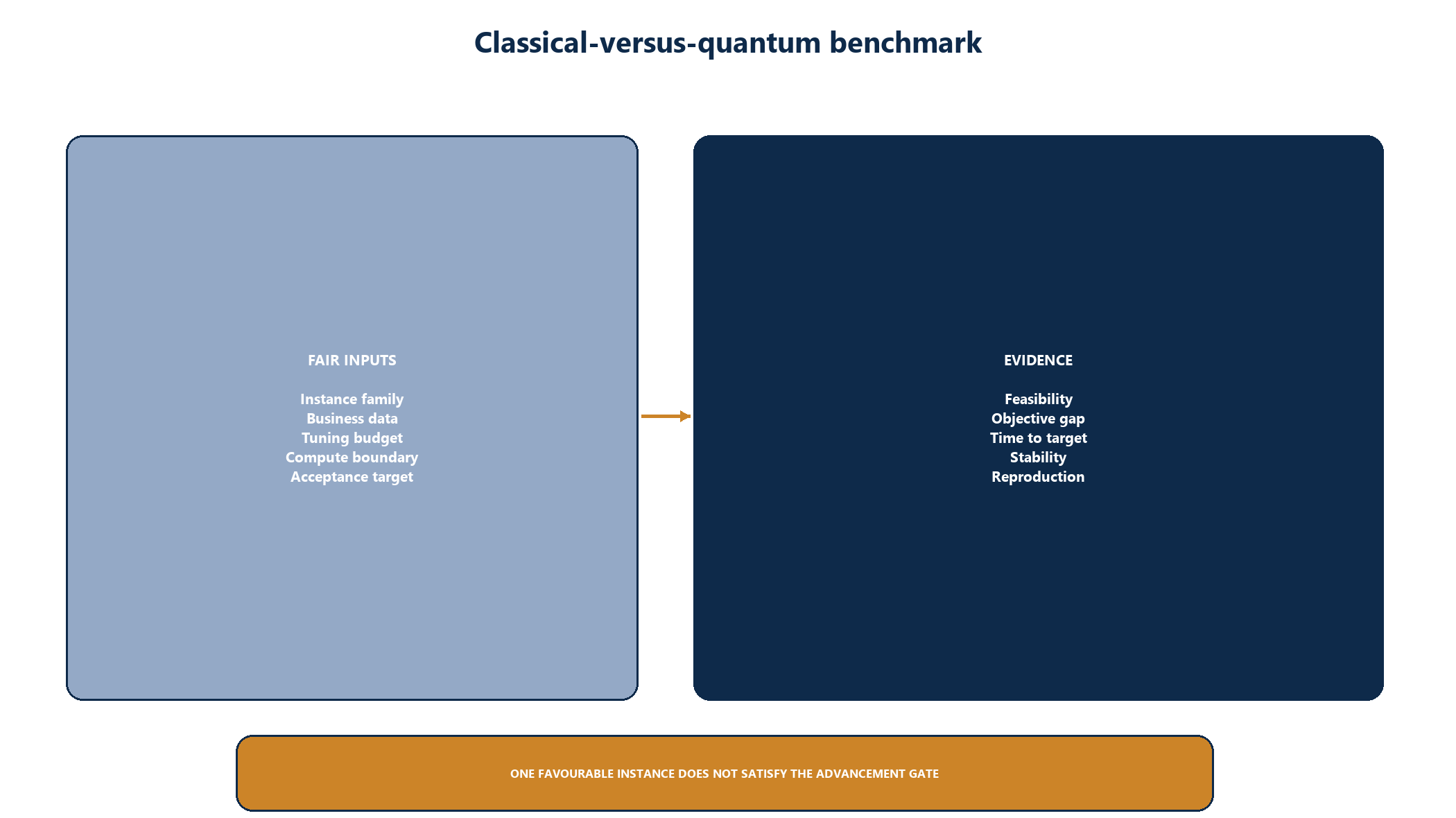
The question is: for a declared family of capital-stack instances, does a challenger produce feasible solutions of better quality, or reach an accepted quality sooner, than the strongest appropriate classical baseline when both receive fair formulation and tuning effort?
Instance families
The suite should contain synthetic controlled instances and permissioned real or realistically transformed instances. It varies instruments, periods, phases, power contracts, scenarios, density, precision and constraint tightness. Easy, medium and hard labels are assigned retrospectively from classical evidence, not from management expectation.
Baselines
Each family receives a tuned MILP or CP-SAT formulation, relevant decomposition, a constructive heuristic and a local-improvement method. Commercial solvers may be included if licensed. Baseline versions, hardware, threads, memory, parameters, warm starts and tuning budget are fixed and recorded.
Challenger accounting
Quantum challenger time includes model conversion, encoding, embedding or transpilation, queue where the chosen metric requires wall-clock service, quantum execution, shots or reads, parameter optimisation, unembedding, repair, validation and repeated runs. Both access cost and energy information are recorded where available and comparable. Missing vendor data is reported as unavailable.
Metrics
Fairness rules
The robust-benchmarking literature recommends application-appropriate formulations, real and hard instances, holistic metrics and equitable hyperparameter effort [28-31].
Advancement gate
A challenger advances from research only if it meets pre-approved thresholds across a representative suite, survives independent replication, adds decision value after full cost and integration, and preserves the audit trail. A single favourable instance does not satisfy the gate.
Figure 7. Classical-versus-quantum benchmark matrix and evidence gates
Source: Matchpoint benchmark framework; benchmarking research [28-31].
Illustrative case, validation and operating model
Illustrative Capital-Stack Case
Scenario status
This entire section is an Illustrative example. The project, parties, prices, amounts, probabilities and outputs are invented to demonstrate the model. They are not a client case, market quote, financing offer or observed benchmark.
Project perimeter
An illustrative sponsor evaluates a three-phase Gulf data-centre campus. Phase 1 is 24 MW, Phase 2 adds 32 MW and Phase 3 adds 48 MW. The sponsor considers equity, a pre-development bridge, senior construction debt, equipment finance and a later term refinancing. Grid power, a renewable PPA, onsite generation and battery support are candidate power components.
Illustrative funding choices
The model minimises discounted all-in funding cost subject to completion, cash, leverage, debt-service, reserve, availability, power and offtake constraints. Equity must fund specified early costs. The construction facility requires approved gates. Equipment finance funds eligible accepted equipment. Refinancing cannot occur before an illustrative stabilisation test.
Illustrative alternatives
Alternative A uses lower initial equity and heavier bridge reliance. It is cheaper in the base case under the invented inputs and becomes infeasible under the nine-month delay because the bridge expires before construction debt availability. Alternative B commits more equity and liquidity earlier. It has a higher base-case carrying cost and remains feasible in the stated delay. Alternative C adds a larger committed facility and a power-contract option; it has the highest stated fees and the lowest reliance on one energisation date.
No numeric solver advantage is stated. A classical solver would establish feasibility, objective and bound for the model. Quantum challengers would receive controlled encodings of selected instance families. The business decision remains an approved choice among transparent alternatives.
Binding constraints
The useful output is often the constraint diagnosis. In the illustrative case, the binding items may include equity-before-debt, interconnection deposit timing, equipment advance rate, minimum liquidity and bridge maturity. A committee can challenge these items and request real counterparty alternatives. The optimiser cannot create commercial terms.
Sensitivity
The paper's scenario chart displays qualitative movement across cost, liquidity, completion and refinancing exposure. It contains no observed client data. Before transaction use, every axis requires approved units, source and tolerance.
Figure 8. Illustrative capital-stack alternatives and binding constraints
Source: Matchpoint Illustrative example; no observed project or solver result.
Governance, Validation And Security
Three lines of control
The first line owns the business model and operating use. Independent model validation challenges data, formulation, code, numerical behaviour, benchmark design and limitations. Internal audit or another independent assurance function evaluates governance and control design. The exact organisational allocation depends on approved policy.
Model-risk standard
Federal Reserve and OCC model-risk guidance emphasises robust development, effective challenge and sound governance [49]. NIST's AI Risk Management Framework provides a broader governance, mapping, measurement and management structure [50]. These sources are applied as control references; legal applicability requires specialist confirmation.
Validation tests
Validation includes unit tests, balance tests, dimensional checks, known-optimum instances, infeasible cases, perturbation tests, dual or bound reconciliation where available, solver cross-checks, seed repetition, penalty sensitivity, encoding precision, repair analysis and independent business review. Every material defect receives an owner and resolution state.
Quantum-specific controls
Quantum tests record provider, backend, calibration context if available, queue and execution timestamps, circuit or embedding, number of shots or reads, parameters, seed, post-processing and raw result reference. Vendor-managed hybrid services record all metadata the service exposes and explicitly state what cannot be observed.
Data protection and confidentiality
Financing terms, tenant contracts, grid correspondence, equipment pricing and credit information may be confidential. Data minimisation, access control, encryption, regional processing, retention, supplier terms and incident response require approval. A public or shared quantum service receives no project data unless the approved security and legal process permits it.
Software supply chain
Open-source packages, solver binaries, cloud SDKs and generated environments are pinned and scanned. NIST's Secure Software Development Framework provides control context [51]. The production repository stores source, lock files, build records and checksums. Secrets remain outside code and reports.
Decision record
The approved decision record contains the considered alternatives, sources, model version, solver runs, validation status, binding constraints, sensitivities, professional advice, conflicts, approvals and reasons for any management override. A solver recommendation never replaces that record.
Quantum-Ready Operating Model
Stage 0: model hygiene
Create canonical objects, identifiers, units, version controls, deterministic calculations and a reconciled classical model. Establish data permissions and decision rights. No quantum work proceeds with unreconciled sources-and-uses or undefined constraints.
Stage 1: research instances
Generate small instances with known optima and progressively harder synthetic instances. Test QUBO, CQM and QAOA mappings on simulators and approved services. Report failures and full resource accounting.
Stage 2: shadow benchmark
Run classical and quantum challengers on permissioned historical or realistic transformed inputs. Outputs remain outside the live transaction process. Independent validators reproduce a sample and assess decision relevance.
Stage 3: analyst support
A validated challenger may propose alternatives to an analyst while the classical production model remains authoritative. The analyst sees lineage, feasibility, objective difference, uncertainty and limitations. All accepted changes are re-solved and validated in the production model.
Stage 4: controlled production component
Only a narrow component with approved evidence, fallback, service-level terms and monitoring can enter production. Examples may include candidate generation for a bounded binary subproblem. A deterministic validator and classical fallback remain mandatory.
Exit and pause criteria
Research pauses if data cannot support the formulation, classical methods solve all material instances within the required time, quantum mapping overhead dominates, feasibility is unreliable, provider metadata is insufficient, confidentiality cannot be approved or expected decision value does not justify cost.
Figure 9. Quantum-readiness roadmap from classical baseline to controlled component
Source: Matchpoint implementation framework; governance and roadmap context [31,46-51].
| Metric | Definition | Decision use |
|---|---|---|
| Feasibility rate | Valid solutions divided by returned samples or runs | Tests constraint control |
| Objective gap | Difference from best verified reference using declared denominator | Tests solution quality |
| Time to target | Total measured time to first accepted-quality feasible result | Tests operational utility |
| Time to solution | Time adjusted for success probability under declared method | Tests stochastic solvers |
| Stability | Distribution across seeds, runs and hardware calibrations | Tests repeatability |
| Scaling | Metric trend across controlled instance size and hardness | Tests growth behaviour |
| Total cost | Service, compute and implementation cost within declared boundary | Tests commercial relevance |
| Explainability | Binding constraints, lineage and reproducible run record | Tests governance readiness |
Implementation gates and limitations
Economics, Capacity And Implementation
Evidence boundary
No Matchpoint or client financial outcome is claimed. Vendor service prices, solver licences and internal effort require current quotes and approved records.
Measurement model
Ninety-day research plan
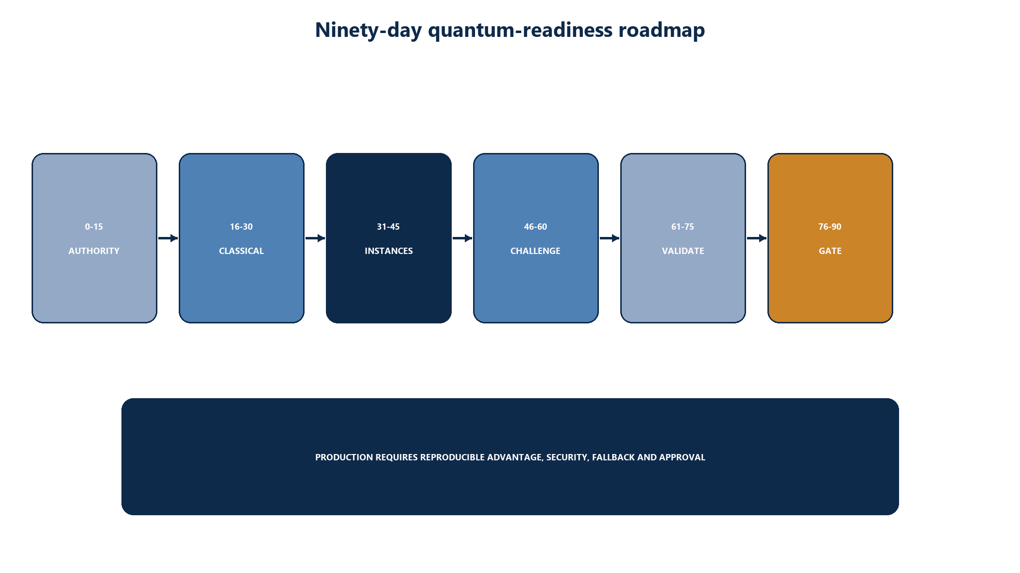
Days 0 to 15: authority and data. Confirm audience use cases, source owners, confidentiality, decision rights, approved classical tools and model-risk governance.
Days 16 to 30: canonical classical model. Build and reconcile a small MILP or CP-SAT instance with deterministic validators, known-optimum tests and business-readable outputs.
Days 31 to 45: instance library. Create controlled tranche, draw, power and integrated instance families. Archive generators, hashes and reference solutions.
Days 46 to 60: D-Wave and QAOA experiments. Build CQM, QUBO and QAOA challengers, starting with simulators and approved test services. Measure the complete resource boundary.
Days 61 to 75: independent validation. Reproduce selected runs, challenge fairness, test penalty and precision sensitivity, and assess whether outputs add decision value.
Days 76 to 90: management gate. Stop, extend research or approve a tightly scoped shadow component. Record evidence, limitations, cost and next acceptance criteria.
Minimum gates
Limitations And Conclusion
Limitations
This paper is a research and operating-design document. It does not provide legal, regulatory, engineering, power-market, environmental, accounting, tax, valuation, credit, investment or quantum-technology advice. Data-centre projects differ by jurisdiction, grid, customer, design, equipment, financing and contract.
The proposed model simplifies construction, power dispatch, tenant credit, tax, accounting, collateral value, refinancing and market execution. Specialist models may need to remain separate and exchange approved boundary values. A compact QUBO may omit detail that is material to underwriting. A high-quality candidate can still be commercially unavailable.
The quantum evidence is evolving and problem-specific. D-Wave and IBM materials describe current products, documentation and roadmaps; capability and roadmap claims from vendors remain vendor-supplied. Peer-reviewed results on MaxCut, SAT, spin models or other benchmarks do not establish advantage on capital-stack optimisation. Hardware noise, embedding, transpilation, parameter training, discretisation, queueing, repair and classical post-processing can alter measured performance.
The worked case and all operating values are hypothetical illustrative examples.
Conclusion
Data-centre capital-stack design is a suitable subject for disciplined optimisation because capital instruments, construction phases, power contracts, reserves and covenant tests form a connected decision system. The business model should begin with controlled source data, explicit authority, deterministic calculations and a well-engineered classical baseline.
Quantum annealing, hybrid CQM and QAOA offer research pathways for selected combinatorial components. Their mathematical fit is testable now. Their transaction value requires a controlled benchmark for this use case. A credible programme compares them with the strongest relevant classical methods, counts the full computation and repair boundary, validates every candidate independently and advances only on pre-approved evidence.
The recommended first implementation is one capital-stack decision, one approved instance library, one classical production model and two bounded challenger tracks. The sponsor and investors retain authority. No Matchpoint or client financial outcome is claimed.
| Gate | Required evidence |
|---|---|
| Business | Named decision, owner, service window and acceptance target |
| Data | Permissioned sources, lineage, freshness and reconciliation |
| Classical | Strong baseline, validation and reproducible run records |
| Quantum | Declared mapping, hardware or service, total accounting and raw outputs |
| Fairness | Equivalent information and equitable tuning budget |
| Security | Approved provider, access, retention and incident controls |
| Validation | Independent feasibility and replication evidence |
| Economics | Observed cost and approved decision-value evidence |
