
1. Degradation is a cash-flow variable
A battery creates value by moving power across time, providing reserve response, supporting capacity obligations and managing network constraints. Each service consumes a combination of power capability, stored energy, availability and state-of-charge flexibility. The same dispatch that earns revenue can reduce future capability. A financial model must therefore price both the immediate gross margin and the lifecycle cost of delivering it.
An annual haircut does not show this relationship. Two projects with the same nominal annual fade can have different economics when one cycles deeply at high temperature and the other provides shallow reserve response. The first may incur earlier augmentation and warranty pressure. The second may preserve energy capacity while still experiencing calendar ageing, auxiliary consumption or availability loss. Debt service depends on the realised path, not the headline assumption alone.
The central modelling question is practical: after each dispatch interval, how much contracted capability remains, what cash flows change, who pays, and what evidence supports the answer? The model should retain enough detail to explain the result to an owner, lender, offtaker, insurer and technical adviser.
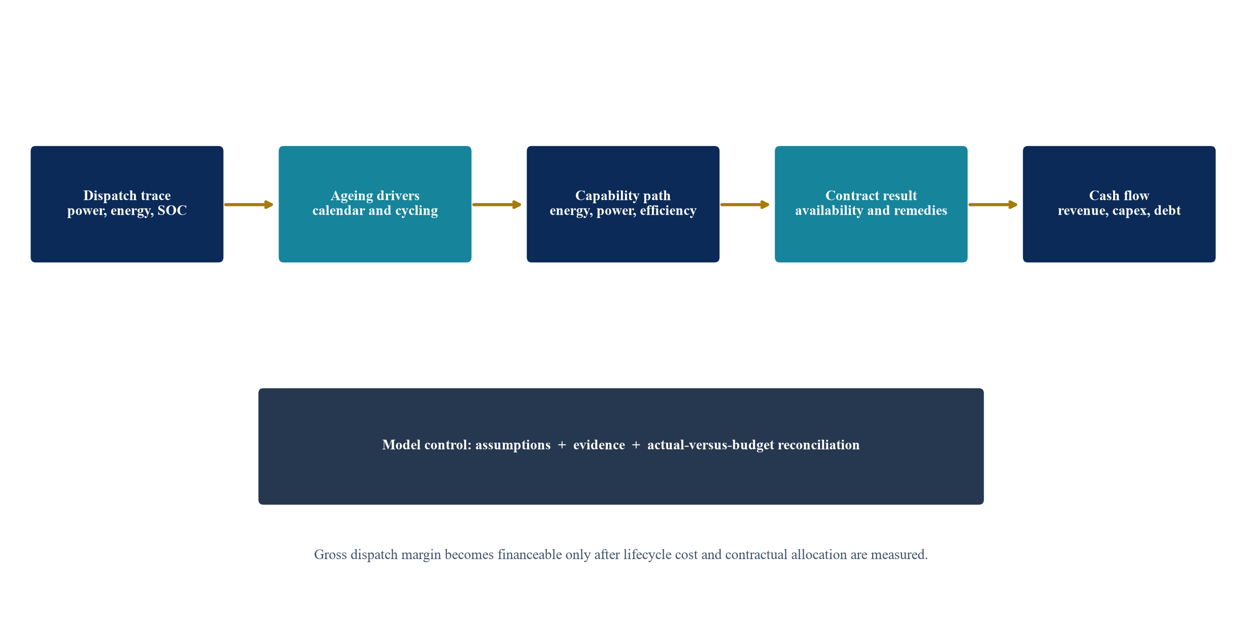
Conceptual framework. Each operating decision affects physical capability, contract performance and cash flow through a traceable sequence.
2. Keep four capability measures separate
Usable energy measures the quantity that can be discharged within defined operating limits. Power measures the rate at which energy can be delivered or absorbed. Round-trip efficiency connects charging energy to delivered energy. Availability measures whether the asset can perform when required. These quantities interact, yet they are not substitutes.
Capacity fade is commonly used for cell ageing. Project revenue may depend more directly on energy delivered at the grid meter, after voltage effects, conversion losses, auxiliaries and operating limits. Sandia reported in August 2026 that using capacity fade in place of energy fade can create a lifetime-prediction error of up to 15 percent in the studied cases. The implication for finance is direct: the model should use the metric that matches the contracted service and settlement boundary.
Power capability can remain adequate while usable energy falls below a duration obligation. A four-hour battery that retains inverter power and loses energy may fail a four-hour capacity test before it fails a power test. Efficiency loss can reduce net market revenue and increase charging cost even when measured capacity remains within warranty. The model should carry all four paths.
3. Calendar ageing continues when the battery waits
Calendar ageing develops with time and is influenced by temperature and state of charge. A battery that is rarely dispatched can still lose capability. NREL's battery-lifespan materials describe predictive models that consider electrochemical, thermal and mechanical modes, storage environment and operating windows. NREL's BLAST suite combines degradation with electrical and thermal performance for real-world profiles.
The financial model should calculate calendar exposure by time interval or by a technically justified approximation. A flat annual rate can be used for a preliminary screen when it is explicitly identified as a simplification. A finance case should test temperature, average state of charge and downtime assumptions that correspond to the site, control policy and thermal-management design.
Calendar ageing also affects construction and commissioning risk. Cells can age between manufacture, delivery, energisation and commercial operation. Long storage periods at adverse state of charge or temperature may consume part of the expected life before revenue starts. Supply and EPC schedules should therefore connect preservation requirements, commissioning tests and baseline capacity measurements.
4. Cycle ageing follows the dispatch profile
Cycle ageing depends on more than the count of charge-discharge events. Depth of discharge, charge and discharge rate, temperature, resting state of charge and partial-cycle sequence can change damage. A shallow ancillary-service pattern can produce many reversals with modest energy throughput. Arbitrage can produce fewer, deeper cycles. Both require an operating trace.
Equivalent full cycles provide a useful normalisation. A common representation divides cumulative discharged energy by rated usable energy. The denominator must be specified: initial nameplate, current usable energy or contracted energy can produce different results. Charging throughput, discharged throughput and total bidirectional throughput should not be mixed without definition.
Equivalent full cycles remain a summary, not a complete ageing model. Two traces with identical throughput can produce different degradation because of temperature, rate and state-of-charge distribution. The project should retain interval data and calculate the warranty measure exactly as the contract defines it.
5. Build a degradation driver ledger
The technical model should record the variables that influence ageing and the variables that determine performance. The financial model should import controlled outputs rather than reconstructing electrochemistry. A driver ledger creates a bridge between the dispatch optimiser, technical adviser and cash-flow model.
Table 1. Degradation driver and financial-treatment ledger
| Driver or measure | Technical meaning | Contract question | Financial-model treatment | Evidence source |
|---|---|---|---|---|
| Calendar time | Elapsed ageing exposure | When does the guarantee clock start? | Time-indexed capability path | Delivery, commissioning and warranty dates |
| Discharged throughput | Energy delivered from the battery | Which meter and losses apply? | Variable degradation cost and cycle budget | SCADA, revenue meter and BMS |
| Equivalent full cycles | Normalised throughput measure | What is the denominator? | Operating-limit test and scenario input | Warranty definition and dispatch trace |
| Depth of discharge | Swing within state-of-charge range | Which bands are permitted? | Damage weighting and optimiser constraint | BMS data and operating protocol |
| C-rate | Power relative to capacity | Are charge and discharge rates limited? | Stress case and performance adjustment | OEM curve and inverter data |
| Temperature | Cell or module thermal condition | Which sensor and exclusions apply? | Calendar and cycle sensitivity | Thermal system and BMS history |
| Usable energy | Deliverable energy within limits | At which point and test conditions? | Revenue capacity and duration compliance | Capacity test protocol |
| Round-trip efficiency | Delivered energy relative to charging energy | Which auxiliaries and meters are included? | Charging cost, revenue and deductions | Contract test and settlement data |
| Availability | Time or intervals capable of service | Which exclusions and notice rules apply? | Revenue deductions and covenant headroom | Outage log and availability report |
General framework. Project definitions should follow the executed warranty, service and revenue contracts.
6. Make the dispatch trace the model's source data
A degradation model should begin with the same interval dispatch used in the revenue model. Market prices, bids and awards determine desired operation. Physical constraints determine feasible operation. The realised trace then determines throughput, state of charge, temperature exposure, efficiency and outages. Parallel revenue and degradation models using different dispatch traces create false precision.
NREL's System Advisor Model supports manual schedules and automated dispatch while accounting for voltage, temperature and degradation. Its documentation illustrates the core control principle: operation, technical performance and replacement timing belong in the same simulation chain. A project can use another validated tool; the integration requirement remains.
The base case should preserve hourly or sub-hourly outputs where market products require them. Annual averages can hide concentrated stress. A battery may earn a large share of annual margin during a small number of volatile periods. Those periods can also produce the most aggressive cycling, temperature or state-of-charge exposure.
7. Choose the degradation method deliberately
Three broad methods are common. A warranty-table method maps cycle count and depth of discharge to retained capacity. An empirical semi-physical model estimates calendar and cycling mechanisms from test data. A machine-learning model learns degradation patterns from observed curves. Each has a different evidence requirement and error structure.
Warranty tables are transparent and contract-relevant. They can be coarse and may not represent the project's temperature, rate or mixed duty cycle. Semi-physical models can explain drivers and extrapolate within validated bounds. They require cell-specific calibration and careful scaling to the system. Machine learning can detect complex patterns; the training domain and uncertainty must be visible.
Argonne researchers demonstrated early-life prediction of capacity-fade curves using the first 100 cycles of a public lithium iron phosphate dataset. The reported errors varied by output, including higher error for rollover-cycle and end-of-life prediction than for curve fit. A finance model should therefore carry prediction uncertainty and avoid treating a point estimate as a guarantee.
8. Align chemistry, cell design and operating regime
Lithium iron phosphate and nickel-manganese-cobalt systems can have different ageing behaviour, safety characteristics and operating limits. Cell design, supplier, manufacturing lot and control software matter within a chemistry. A generic industry curve should not displace project-specific evidence.
The model should identify cell supplier, module and rack configuration, inverter topology, thermal system and battery-management logic. If procurement permits multiple suppliers, each approved configuration needs a performance representation or a conservative common case. Substitution rights should preserve bankability through testing, warranty and model updates.
Changes during construction or augmentation can create a mixed fleet. New cells may have different voltage, capacity or control characteristics from older cells. The augmentation plan should address compatibility, segmentation and measurement. The financial model should not assume that one unit of new nameplate capacity restores one unit of contracted usable energy without integration loss.
9. Define the measurement boundary
Performance can be measured at cell, module, rack, inverter or grid meter. Each boundary includes different losses and auxiliaries. Warranty capacity at the DC block may not equal contracted energy at the point of interconnection. Round-trip efficiency can include or exclude heating, cooling, controls and transformer loss.
The model should contain a loss bridge from cell capability to settled service. Each item needs an owner, test method and data source. The bridge should reconcile nameplate, operating reserve, state-of-charge limits, conversion loss, auxiliary load, downtime and contractual exclusions.
A fixed loss assumption should be tested against load and temperature. Auxiliary consumption can rise during hot periods or low utilisation. Efficiency can vary with power. The model needs enough granularity to avoid overstating net energy and understating charging cost.
10. Model energy fade and capacity fade consistently
Capacity fade records loss of charge storage under specified test conditions. Energy fade also reflects voltage behaviour across discharge. Sandia's 2026 research highlights that the two measures can diverge when cell results are scaled to system life. A project-level model should identify which curve drives usable energy.
The distinction affects augmentation. If the contract promises megawatt-hours delivered over a duration, energy fade is economically relevant. If the warranty tests ampere-hours under laboratory conditions, a conversion is required. The conversion should account for voltage, temperature, state of charge, power and balance-of-system losses.
The model should retain both the technical observation and the financial proxy. Replacing one with the other prevents later reconciliation. Actual capacity tests, energy tests and meter data can then update the appropriate state variable.
11. Treat efficiency as a degrading asset attribute
Round-trip efficiency determines how much charging energy is required for each unit delivered. Lower efficiency increases charging cost and can reduce net market revenue. It can also trigger performance deductions. An SEC-filed energy-storage agreement provides a schedule in which a guaranteed efficiency rate declines by 0.22 percentage points per contract year from an initial 84.5 percent, illustrating that contract tests can contain a time path rather than one static threshold.
The model should distinguish technical efficiency from contractual efficiency. The technical model may use AC or DC conversion curves and auxiliary loads. The contract may define meter locations, test windows, exclusions and calculation conventions. Cash deductions follow the contract definition.
An Energy Vault filing describes a monthly floor adjusted for availability and round-trip efficiency, with an annual true-up. This structure shows how performance can affect otherwise contracted cash flow. The finance model should calculate the same adjustment sequence and timing.
12. Make warranty terms machine-readable
A warranty should be translated into model constraints. Relevant fields include commencement, term, warranted energy, power, efficiency, availability, throughput, cycle limits, temperature bands, state-of-charge bands, excluded events, measurement method, notice, cure, remedy, liability cap and supplier security.
Fluence's public filings describe assurance and service-type warranties and arrangements to maintain battery capacity above a threshold or perform fixed augmentations. They also describe performance liquidated damages when guaranteed thresholds are missed. These disclosures establish contract mechanisms rather than project terms. Each project must model its executed documents.
The model should compare each simulated interval or test period with the applicable condition. A warranty curve without compliance logic can overstate recovery. A claim may fail because dispatch breached a limit, data are missing, notice was late or the loss falls within an exclusion.
13. Separate technical loss from warranty recovery
Technical degradation occurs whether or not a claim is recoverable. Warranty recovery is a contingent cash flow with timing, evidence and counterparty risk. The base financial model should first recognise physical performance. It should then apply contract recovery as a separate layer.
This separation avoids two errors. The first treats warranty coverage as if degradation does not occur. The second assumes an immediate cash reimbursement equal to the lost revenue or replacement cost. Remedies may be repair, replacement capacity, service, liquidated damages or a capped payment after testing and cure.
Recovery timing can affect debt service. A replacement delivered twelve months after a failed test does not restore cash flow during the delay. The model should carry a receivable only when recognition is justified and should stress dispute, delay and supplier credit.
14. Create a governed degradation budget
The project should approve an annual and cumulative degradation budget. The budget can express equivalent full cycles, throughput, time at high state of charge, temperature exposure and expected capability. Dispatch decisions then consume budget alongside market opportunity.
The optimiser should include a marginal degradation cost or shadow price. This price converts future capability loss and augmentation cost into a current dispatch constraint. It need not be perfectly precise to improve discipline. It should be reviewed as operating evidence accumulates.
Budget governance should define authority to exceed limits. A volatile market event may justify additional cycling when net value remains positive. The decision should record expected gross margin, incremental lifecycle cost, warranty effect, covenant headroom and responsible approver.
15. Convert degradation into a marginal cost
The simplest marginal cost divides the present value of lifecycle expenditure by permitted lifetime throughput. A stronger method calculates the change in present value caused by an incremental dispatch. It includes lost future revenue, earlier augmentation, additional charging loss, maintenance and warranty consequences.
The marginal cost will vary with state of charge, temperature, depth and remaining life. A single annual value can be used as a floor for routine optimisation, with adders for stressful conditions. The model should show how the number was derived and how often it is recalibrated.
Merchant dispatch should be tested on net spread after charging energy, market fees, variable operations cost and degradation cost. Ancillary-service bids should include expected activation and state-of-charge restoration. Capacity revenue should include the cost of preserving deliverable energy for the obligation.
16. Model augmentation as an operating decision
Augmentation adds cells, modules or blocks to restore capability. It can be scheduled at fixed dates, triggered by a threshold or optimised dynamically. Sandia's energy-storage handbook distinguishes initial oversizing and later augmentation. Oversizing can simplify integration and protect early performance; augmentation can benefit from future cost reductions and observed ageing.
Augmentation is not only a battery purchase. It can require engineering, transport, labour, shutdown, control-system changes, testing, permits, spares and balance-of-system capacity. Space, electrical design and fire-safety approvals can constrain the plan. The financial model should include all-in installed cost and downtime.
The decision should compare the present value of augmentation with revenue preserved, performance deductions avoided and residual value created. It should also test whether a smaller addition postpones a larger intervention. A rule that automatically restores nameplate capacity every year can hide uneconomic spending.
17. Distinguish oversizing, augmentation and replacement
Initial oversizing installs additional capacity before operation. Augmentation adds capacity while the original asset remains. Replacement removes or retires degraded equipment and installs new equipment. The three strategies have different capex timing, tax, warranty, integration and residual-value effects.
Oversizing increases day-one capital and may leave capacity unused early in life. It can reduce future construction interfaces and protect contractual capability. Augmentation defers capital and learns from actual degradation; it introduces execution risk. Replacement can reset part of the fleet and may recover salvage value; it can require a longer outage.
The model should present the strategies on a common net-present-value basis with the same dispatch and performance obligation. Financing documents should permit the chosen approach and retain lender control over material expenditure and asset removal.
18. Build three linked ledgers
The technical ledger records dispatch, state of charge, temperature, throughput, efficiency, availability and capability. The contract ledger applies warranties, performance guarantees, deductions, liquidated damages and claims. The financial ledger records revenue, charging cost, maintenance, augmentation capex, recoveries, tax, debt service and residual value.
Every material cash flow should trace back to a technical or contractual event. An augmentation payment should identify the capability threshold and installed quantity. A revenue deduction should identify the test, measurement period and exclusion. A warranty recovery should identify the claim basis and assumed collection date.
Linked ledgers make diligence and model audit practical. They also reduce the risk that one technical assumption is embedded differently in revenue, capex and covenant calculations.
19. Illustrative 100 MW and 400 MWh model
Consider a hypothetical 100 MW, 400 MWh battery with a fifteen-year operating horizon. The example assumes an initial installed cost of USD 120 million, 65 percent senior debt, contracted and merchant revenue, and a minimum four-hour delivery obligation. These figures are illustrative modelling inputs and do not represent a market quote or project.
Three cases use the same revenue opportunities and different degradation paths. The controlled case limits deep cycling and maintains moderate state of charge. The intensive case pursues more arbitrage and incurs faster energy fade. The adverse case combines higher temperature, lower efficiency and delayed augmentation. Augmentation occurs only when its present value is positive and required liquidity is available.
Table 2. Hypothetical degradation and finance cases
| Measure | Controlled dispatch | Intensive dispatch | Adverse execution |
|---|---|---|---|
| Annual discharged throughput | 110,000 MWh | 165,000 MWh | 150,000 MWh |
| Average equivalent full cycles | 0.75 per day | 1.13 per day | 1.03 per day |
| Year-10 usable energy before augmentation | 78% | 69% | 63% |
| Year-10 round-trip efficiency | 84% | 82% | 79% |
| Augmentation timing | Years 8 and 12 | Years 6, 9 and 12 | Planned year 7; delayed to year 9 |
| Nominal augmentation expenditure | USD 14m | USD 24m | USD 29m |
| Minimum DSCR in modelled downside | 1.34x | 1.19x | 0.96x |
| Year-15 residual-value basis | Continuing contracted capability | Merchant capability after planned augmentation | Recovery case after delayed intervention |
Illustrative assumptions only. Figures are not forecasts, market terms or observed project data.
20. Read the illustrative result carefully
The intensive case earns more early gross margin and consumes more capability. Its additional revenue is not free cash flow when augmentation occurs earlier and debt-service headroom falls. The result depends on the assumed market spreads, degradation function and capex curve. A different price path can reverse the ranking.
The adverse case shows timing risk. A technically justified augmentation can fail to protect lenders when procurement, permits or liquidity delay installation. Revenue deductions and efficiency losses occur before capacity returns. The financing plan must therefore include trigger lead time and reserve funding.
The example supports a decision rule: approve a dispatch strategy after comparing incremental revenue with the present value of degradation, contractual effects and liquidity demand. The model should show both the economic optimum and the financeable operating envelope.
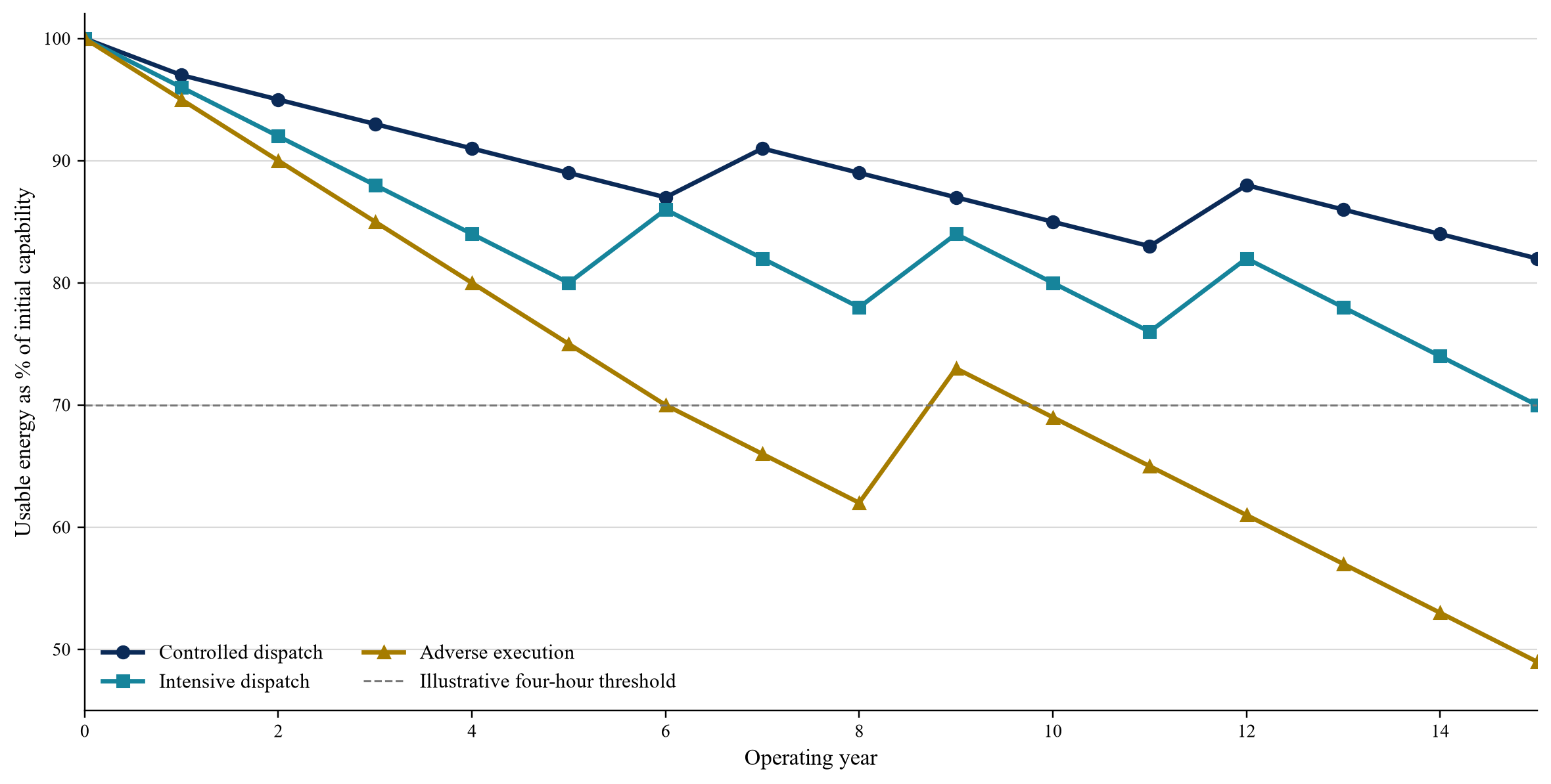
Illustrative scenarios only. Paths are constructed for framework demonstration and do not represent observed projects or forecasts.
21. Size debt against post-degradation capability
Debt sizing should use the capability and cash-flow path after degradation, losses, downtime and augmentation. A lender should not underwrite initial nameplate revenue across the full tenor. Contracted revenue may also decline when performance deductions apply.
The base case should contain a technically supported degradation path and a funded augmentation plan. The downside should stress faster fade, lower efficiency, reduced availability, higher augmentation cost, delay and warranty non-recovery. A tail case should test nonlinear deterioration or an early module problem.
Debt service coverage should be calculated before and after reserve funding. A project can report adequate operating cash while accumulating an unfunded augmentation obligation. Restricted cash, lifecycle reserves and distribution tests should preserve the ability to intervene before contracted performance fails.
22. Fund the lifecycle reserve
A lifecycle reserve can be funded at closing, through periodic cash sweeps, by letter of credit or through committed sponsor support. The choice depends on augmentation timing, counterparty strength, debt tenor and market risk. A reserve based only on expected cost may be insufficient when equipment price, freight, labour or integration cost rises.
The funding schedule should follow decision lead time. Cash may be required before the capability threshold is breached because procurement and installation take time. Release conditions should require completed performance testing and updated forecasts rather than calendar passage alone.
Unused reserve belongs in the terminal model. It can fund later replacement, repay debt or distribute to equity according to the documents. The model should prevent the same cash from supporting both debt service and future augmentation.
23. Link covenants to measurable capability
Financial covenants can be late indicators of degradation. Operational covenants provide earlier warning. Suitable measures include usable energy, efficiency, availability, cumulative throughput, state-of-charge compliance, temperature excursions, warranty headroom and forecast augmentation funding.
Testing frequency should match volatility and contract measurement. Monthly operational reporting can support quarterly lender review. Annual capacity tests alone may miss rapid change. Continuous BMS data require validation and clear treatment of missing or revised values.
A breach should lead to a proportionate response: investigation, dispatch restriction, reserve top-up, remediation plan, distribution lock-up or default for severe unresolved failure. The documents should preserve owner and lender access to data and control systems.
Table 3. Degradation monitoring and finance-control matrix
| Indicator | Evidence | Early-warning question | Financial consequence | Governance response |
|---|---|---|---|---|
| Usable energy | Controlled capacity or energy test | Is capability below the approved path? | Revenue loss and earlier augmentation | Technical review and forecast reset |
| Round-trip efficiency | Revenue meters and test protocol | Are charging costs or deductions rising? | Lower net margin and contracted payment | Dispatch and thermal review |
| Equivalent full cycles | Validated dispatch data | Is lifecycle budget being consumed early? | Higher marginal cost and reserve demand | Restrict or reprice dispatch |
| Temperature exposure | BMS and thermal logs | Are excursions persistent or concentrated? | Faster ageing and warranty risk | Root-cause plan and operating limit |
| Availability | Outage and maintenance records | Is downtime technical or operational? | Capacity and toll deductions | Maintenance cure and spares action |
| Warranty headroom | Compliance calculation | Are operating limits close to breach? | Reduced recovery value | Notice, evidence preservation and control change |
| Augmentation coverage | Cost estimate, reserve and schedule | Is funding available before the trigger? | Liquidity shortfall and DSCR pressure | Reserve top-up or sponsor support |
| Model error | Actual-versus-budget reconciliation | Is forecast bias persistent? | Mispriced dispatch and valuation | Independent recalibration |
General framework. Thresholds and remedies depend on project documents and technical advice.
24. Treat uncertainty as a distribution
Degradation is uncertain because cell variability, site conditions, controls and future dispatch differ from test conditions. A finance model should use scenarios or probability distributions rather than one deterministic curve. The choice should match data quality and decision purpose.
Relevant uncertainties include calendar rate, throughput damage, efficiency, temperature, nonlinear knee onset, downtime, augmentation cost, procurement delay and warranty recovery. Correlations matter. High temperature can reduce efficiency and accelerate ageing while increasing auxiliary load.
The model should report percentile outcomes or clearly defined cases for capability, augmentation date, reserve sufficiency, debt service and residual value. A confidence interval without its model domain can mislead. The technical adviser should identify where extrapolation begins.
25. Stress the nonlinear knee
Lithium-ion degradation can accelerate after a knee point. An early-life linear trend may therefore overstate remaining life. Argonne's capacity-fade research treats rollover-cycle prediction as a distinct output, illustrating the need to monitor curve shape as well as average loss.
A knee stress can apply an additional capability decline after a trigger defined by time, throughput or observed state of health. The trigger and severity are scenario assumptions unless supported by project-specific evidence. The model should show the cash consequence of detection delay.
An operating strategy can preserve option value when uncertainty is high. Moderate dispatch, diagnostic testing and staged augmentation may produce more value than maximising near-term revenue if they reduce the chance of irreversible loss or preserve warranty recovery.
26. Reconcile actual performance each month
The project should compare actual throughput, cycles, temperature, state of charge, efficiency, availability and capability with budget. Variance should be separated into dispatch choice, market activation, weather, equipment, outage and measurement effects.
The forecast should update prospectively. Historical assumptions should remain archived so the board and lenders can assess model error. A silent overwrite destroys learning and can conceal deterioration. Versioned technical and financial baselines create an audit trail.
Reconciliation should also test revenue quality. Higher gross revenue accompanied by faster capability loss may reduce value. The report should show net margin after degradation allocation and the change in augmentation timing.
27. Govern optimiser incentives
An optimiser paid on gross market revenue can prefer aggressive dispatch. An owner funding augmentation can prefer asset preservation. Incentives should reward net value within lifecycle limits. The commercial agreement can include a degradation charge, throughput price, shared augmentation cost or performance adjustment.
The optimiser should receive current technical constraints and should return a complete dispatch record. The owner needs override rights for safety, warranty and approved lifecycle limits. Override use should be logged because excessive restriction can also destroy value.
Compensation can use a benchmark for feasible market value after constraints. The benchmark should be reproducible and should not assume information unavailable in real time. Disputes over counterfactual revenue should not delay critical asset protection.
28. Price the warranty counterparty
Warranty value depends on the supplier's ability and willingness to perform. The model should consider term, liability cap, parent support, insurance, security, governing law, claim process and surviving obligations. A technically strong warranty from a weak counterparty can have limited finance value.
Fluence filings show that warranty liabilities and performance guarantees are recognised financial exposures. Public amounts for one supplier do not determine another project's recovery. They demonstrate that warranties create real obligations with estimation risk.
The lender case should apply collection delay and recovery haircuts where justified. Replacement capacity may be more valuable than cash when market access and integration are scarce. Step-in rights should preserve claims after enforcement.
29. Account for augmentation and warranty correctly
Augmentation expenditure can create or improve an asset; maintenance restores existing condition. Warranty reimbursement may reduce cost or be recorded separately depending on the arrangement and accounting policy. Tax treatment can differ by jurisdiction and component.
The financial model should maintain book, tax and cash ledgers. Depreciation should follow the recognised asset and useful life. Deferred tax and incentive eligibility should be reviewed when substantial equipment is added after commercial operation.
Accounting presentation should not change project economics, yet it can affect reported ratios, distributions and covenant definitions. Executed finance documents should state whether augmentation capex, warranty proceeds and reserve movements are included in relevant calculations.
30. Value the residual asset by remaining capability
Residual value should reflect deliverable service after remaining degradation, required capex, contract position and market access. Initial nameplate cost is not a valuation anchor at the end of life. The asset may have continuing grid rights, land, connection, control systems and reusable balance of plant even when battery blocks require replacement.
The valuation should separate existing battery capability from the option to repower. A repowering case needs future equipment cost, outage, permits, integration and financing. A salvage case needs removal, transport, recycling and liability assumptions.
Second-life value should be included only with evidence for condition, market, certification and transaction cost. The model should carry decommissioning and recycling obligations even when salvage value is assumed.
31. Diligence the degradation model
Technical diligence should review cell data, ageing method, scaling, dispatch trace, thermal assumptions, controls, test protocols, warranty alignment and augmentation design. Commercial diligence should review revenue products, operating constraints and optimiser incentives. Financial diligence should trace every material output into cash flow and covenants.
The data room should include source files, version history, model code or calculation logic, validation results, BMS schema, commissioning tests, operating history, warranty, service agreement, augmentation plan, cost estimates and claims. Summary presentations do not replace source evidence.
An independent reviewer should reproduce selected outputs. Useful tests include one-day dispatch, one-year throughput, capability at a warranty milestone, augmentation trigger, cash reserve movement and DSCR response. Differences should be resolved before financing.
32. Use a six-gate model review
Gate one verifies input provenance: cell, system, site, dispatch and contract data. Gate two verifies technical logic: calendar, cycle, temperature, efficiency and capability. Gate three verifies contract mapping: tests, exclusions, remedies and payment effects.
Gate four verifies lifecycle actions: oversizing, augmentation, replacement and decommissioning. Gate five verifies cash flow: revenue, charging cost, capex, reserve, tax, debt service and residual value. Gate six verifies governance: approvals, reporting, recalibration and change control.
The investment committee should receive exceptions at each gate. Approval should state which assumptions are supported, which are scenario inputs and which remain conditions precedent. The model becomes an operating control after closing.
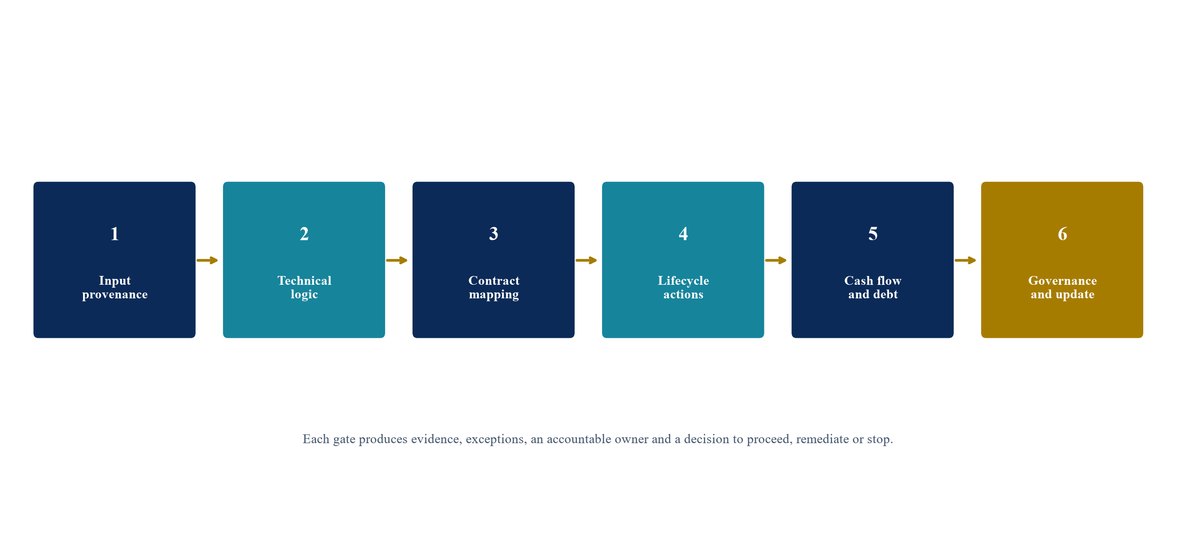
A financeable model links technical evidence to contracts, lifecycle actions, cash flow and ongoing governance.
33. Decision rules for owners and lenders
The owner should approve dispatch only within the modelled lifecycle envelope or through a recorded exception. The optimiser should price degradation in bids. The technical manager should update capability and warranty headroom. The finance team should maintain reserve sufficiency and covenant forecasts.
Lenders should require the integrated model, data rights, independent testing, funded lifecycle plan and change control. They should review aggressive merchant assumptions together with the degradation they create. A higher gross-revenue case is not a better debt case when it reduces minimum coverage or creates unfunded capex.
Boards should receive a compact dashboard: net dispatch margin after degradation cost, capability against budget, efficiency, throughput, temperature exceptions, warranty headroom, augmentation readiness, reserve coverage and downside DSCR. These measures connect operations to enterprise value.
34. Limitations and research agenda
Degradation models are approximations. Laboratory data may not represent field conditions. Cell results may not scale linearly to modules and systems. Future dispatch, temperature, maintenance and software can differ from the base case. Contract recovery and equipment cost can change.
The illustrative cases in this paper are constructed examples. They do not estimate a representative project's return or predict a specific technology. No universal marginal degradation cost, cycle limit or augmentation schedule follows from them.
Further research should compare predicted energy fade with metered system output across operating fleets; test how optimiser incentives affect lifecycle value; improve uncertainty propagation from cell to project finance; and develop standard evidence for augmentation, warranty and lender monitoring.
35. Conclusion
Battery degradation belongs inside dispatch economics, financing and valuation. A single annual haircut cannot explain how operating decisions consume capability or how contracts allocate the result. The financial model should preserve the dispatch trace and carry separate paths for usable energy, power, efficiency and availability.
The proposed framework connects ageing drivers to performance tests, warranty, augmentation, cash flow and debt service. Three linked ledgers preserve the distinction between physical loss, contractual recovery and expenditure. Scenario analysis captures uncertainty, knee risk, cost escalation and delay.
A governed degradation budget turns the model into an operating control. Actual performance is reconciled with assumptions, optimiser incentives reflect lifecycle cost, reserves fund timely intervention and lenders receive early warning. Every cycle then has an explicit economic meaning rather than an invisible claim on future value.
References
- National Renewable Energy Laboratory, Battery Storage, System Advisor Model, accessed 28 September 2026. https://sam.nrel.gov/battery-storage.html
- National Renewable Energy Laboratory, Battery Lifespan and BLAST Battery Lifetime Analysis and Simulation Tool Suite, accessed 28 September 2026. https://www.nrel.gov/transportation/battery-lifespan.html
- Nicholas DiOrio, Aron Dobos, Steven Janzou, Aldo Nelson and Blake Lundstrom, Technoeconomic Modeling of Battery Energy Storage in SAM, NREL/TP-6A20-64641, September 2015. https://www.nrel.gov/docs/fy15osti/64641.pdf
- Kandler Smith, Aron Saxon, Matthew Keyser, Blake Lundstrom, Ziwei Cao and Albert Roc, Life Prediction Model for Grid-Connected Li-Ion Battery Energy Storage System, NREL/CP-5400-67102, 2017. https://www.nrel.gov/docs/fy17osti/67102.pdf
- Sandia National Laboratories, Using Energy Fade, Not Capacity Fade, Can More Accurately Predict How Long Energy Storage Systems Will Last, 10 August 2026. https://www.sandia.gov/ess/2026/08/10/research-using-energy-fade-not-capacity-fade-can-more-accurately-predict-how-long-energy-storage-systems-will-last
- U.S. Department of Energy, 2022 Grid Energy Storage Technology Cost and Performance Assessment, August 2022. https://www.energy.gov/sites/default/files/2022-09/2022%20Grid%20Energy%20Storage%20Technology%20Cost%20and%20Performance%20Assessment.pdf
- Sandia National Laboratories, Energy Storage Financing: Operations and Market Strategy, SAND2021-14700, November 2021. https://www.osti.gov/servlets/purl/1866526
- Federal Energy Regulatory Commission, Order No. 841, Electric Storage Participation in Markets Operated by Regional Transmission Organizations and Independent System Operators, 15 February 2018. https://www.ferc.gov/media/order-no-841
- Fluence Energy, Inc., Annual Report on Form 10-K for the year ended 30 September 2025, filed 25 November 2025. https://www.sec.gov/Archives/edgar/data/1868941/000186894125000081/flnc-20250930.htm
- Fluence Energy, Inc., Quarterly Report disclosures on product performance guarantees, warranties and capacity guarantees for the period ended 30 June 2026. https://www.sec.gov/Archives/edgar/data/1868941/000186894126000029/R21.htm
- Energy Vault Holdings, Inc., Tolling and power-purchase agreement revenue disclosures for the period ended 30 June 2026. https://www.sec.gov/Archives/edgar/data/1828536/000182853626000101/R9.htm
- SEC-filed Energy Storage Agreement, storage-guarantee efficiency schedule and liquidated-damages mechanism, filed 2025. https://www.sec.gov/Archives/edgar/data/1817004/000149315225024405/ex10-1.htm
- Saurabh Saxena, Logan Ward, Joseph Kubal, Wenquan Lu, Susan Babinec and Noah Paulson, A Convolutional Neural Network Model for Battery Capacity Fade Curve Prediction Using Early Life Data, Argonne National Laboratory, 2022. https://www.osti.gov/servlets/purl/1910034
- Lawrence Berkeley National Laboratory, Solar and Storage Operations, project-level dispatch and market-value research, accessed 28 September 2026. https://emp.lbl.gov/utility-scale-storage
- International Renewable Energy Agency, Renewable Power Generation Costs in 2024, July 2025. https://www.irena.org/Publications/2025/Jul/Renewable-Power-Generation-Costs-in-2024
About the Author
Chennakeshav (CK) is a corporate finance and investment banking executive with 25+ years of global experience in deal origination, structuring and execution across M&A, growth capital and corporate strategy. He has led value-creation mandates for founders, corporates and funds — bridging the boardroom view to hands-on execution and close.
His career spans Morgan Stanley, HSBC, Lloyds Banking Group, EWEC, ADQ portfolio companies and Emirates Growth Fund, across TMT, real estate, fintech, deeptech, cleantech, infrastructure and energy. He has partnered with C-suite leaders, private equity and venture funds, sovereign wealth funds and family offices to finance complex fund raises and scale-up ventures, and has led M&A due diligence, post-merger integration and business-transformation initiatives to create value.
At Matchpoint Partners he is Managing Partner, leading the firm's corporate finance, M&A and capital-raising practice. He holds an MBA from London Business School, an engineering degree from VTU and a Master of Laws (LLM, in progress) from UCL London.
An active start-up mentor, CK mentors at Techstars, DIFC FinTech Hive, Startup Grind, Founder Institute and IN5, serves as Entrepreneur Mentor in Residence (EMiR) at London Business School, and judges the Entrepreneurship World Cup.
LinkedIn: https://www.linkedin.com/in/ckadya/
Profile: https://www.matchpoint-partners.com/team/ck-adya.html
