

1 The board's decision and the evidence boundary
An acquisition board needs information about customer continuity, critical capabilities, operating delivery and the benefits assumed in its investment case. Consolidated financial reports and operational records describe different parts of that picture and can become available on different dates. This paper examines which operational warnings deserve investigation, the thresholds at which they should be escalated and the evidence needed to evaluate their economic contribution.
We frame monitoring as a detection decision with costs for missed deterioration and investigations. An undetected issue can continue to affect customers, staff, service or cash. An alarm consumes attention and may prompt an expensive response. The constructed experiment compares detection regimes on the same population and reports avoided leakage after a stated false-investigation cost. The financial and operational results remain conditional on every authored input.
This study uses no observed acquisition-level workstream or alarm cohort. The research contribution is an explicit experimental design and a practical recording framework. The simulation generates 20,000 test acquisitions from stated assumptions and tests how detection rules behave within that world. The proposed transaction study would require separate data-access, governance, measurement and evaluation work before any empirical claims could be made.
A jurisdiction-specific oversight example comes from the UK Corporate Governance Code 2024. For companies in its stated commercial-company or closed-ended-investment-fund listing categories, Provision 29 addresses monitoring and annual review of risk management and internal controls, including material financial, operational, reporting and compliance controls. Its enhanced provisions apply to financial years beginning on or after 1 January 2026. [14] The Code supplies no integration-indicator thresholds. The practical tools proposed here address the evidence an acquisition board could retain within its own applicable governance framework.
2 Define onset, financial effect and detection
We define value leakage as the monthly shortfall of delivered contribution against the planned contribution that is caused by a specific integration failure, measured as a percentage of one month of plan. A leak has an operational onset, the month the causal event occurs, and a financial effect that begins some months later. A miss is a quarter in which the reported variance to plan falls below a stated materiality line. Detection is the date at which a rule raises an alarm and the information is available to the board.
The distinction between onset, financial effect and detection date is the central device of the paper. A leading indicator is useful only to the extent that its detection date precedes the date at which the financial statements would show the same problem. That lead is the product of three separate quantities: the lag between cause and financial effect, the delay before an indicator crosses its threshold, and the reporting delay of the financial alternative. Table 1 sets out the definitions used throughout.
| Term | Definition used | Why it matters |
|---|---|---|
| Operational onset | Month in which the causal event occurs, for example loss of a key-account owner | Starts the detection clock |
| Financial effect | Month in which reported variance begins to move because of the event | Date at which accounts could first show it |
| Value leakage | Cumulative shortfall to plan caused by the event, % of one month of plan | The quantity to be protected |
| Alarm | A rule crossing its calibrated threshold, with the accumulator reset after the crossing | Triggers an investigation |
| True alarm | An alarm raised at or after the onset of an event the indicator points to | Counts toward detection |
| False alarm | Any other alarm, including every alarm from a measure unrelated to any event | Costs time and credibility |
| Miss | A quarter whose reported variance is below minus 5% of plan | The financial outcome an alarm should precede |
MatchPoint definitions for this paper. Proposed records; they are not findings about any transaction.
3 Quarterly reporting clocks and earlier management information
The current U.S. Form 10-Q specifies ordinary filing deadlines of 40 days after quarter end for large accelerated and accelerated filers and 45 days for other registrants, for the first three fiscal quarters. [1] These are filing deadlines. Companies can provide earlier internal information, and the form does not prescribe when a private acquirer prepares management accounts. The SEC page for its May 2026 semiannual-reporting initiative identifies that instrument as a proposed rule. [13] Its proposal status should be kept separate from the current form requirements. Regulation S-X permits unaudited interim financial statements and requires independent-accountant review before Form 10-Q filing. [15] The assurance status should therefore be described precisely.
The experiment uses a quarterly series available 1.5 months after quarter end, a deliberately stated reporting assumption. Ignoring any lag before the financial effect and any detection threshold, an event in month one can first enter a quarter ending in month three, available in month 4.5 under this clock. An event in month three enters the same report. The reporting delay therefore depends on the event's position within the quarter. A financial-effect lag, a small first-period loss or a threshold that is not crossed can delay detection further.
The 45-day deadline motivates one reporting-clock scenario; it supplies no minimum information delay and no observation of a board's actual access. The model also tests monthly accounts and faster financial-report availability. For an empirical study, retain the date on which each comparison series was genuinely available to the decision-maker. A published filing date cannot stand in for that date when an internal management pack arrived earlier. The simulation's eight-quarter schedule is a management-reporting comparator. It includes fourth quarters, for which Form 10-Q is not required. [1]
4 Acquisition accounting and operating evidence
Acquisition accounting and operating delivery have different measurement purposes. Where initial acquisition accounting is incomplete, AASB 3 paragraphs 45-47 permit provisional amounts and adjustments for information about facts existing at the acquisition date. The measurement period ends when the needed information is obtained or found unobtainable and cannot exceed one year from acquisition. [2] The applicable compilation and reporting period must be checked for the entity concerned. These provisions do not date the onset of operating problems or establish when integration leakage is most likely.
AASB 3 paragraph B64(q) addresses acquiree revenue and profit or loss since acquisition and specified combined-entity information as if the acquisition occurred at the start of the annual period. Its impracticability provision requires an explanation; B65 addresses collectively material combinations. AusC1 exempts entities using the specified Tier 2 simplified disclosures from these paragraphs. [2] Management can maintain additional internal disaggregation after consolidation, so an aggregate external disclosure does not establish that a board lacks separate operating records.
The Australian standard is cited as an official source for the specified accounting requirements. Each reader must apply the reporting framework and version governing its entity. A warning system should keep its operating definitions and baseline versions traceable while finance records purchase-accounting changes separately. This supports a reconciliation between the approved deal case, revised accounting amounts and actual delivery without treating those records as interchangeable.
The reporting and measurement sources in Table 2 establish particular clocks and disclosure requirements. The source scope is explicit. None supplies a universal private-company reporting lag, validates a leading indicator or establishes that the accounting measurement period predicts operating losses.
| Clock or record | Source statement | Limit of the source |
|---|---|---|
| Quarterly filing | Form 10-Q due 40 days (large accelerated and accelerated filers) or 45 days (others) after quarter end; none for the fourth quarter [1]; semiannual option proposed [13] | Public-company rule; private accounts differ |
| Measurement period | Provisional acquisition amounts may be adjusted; period not to exceed one year from acquisition date [2] | Period-specific AASB compilation; operating losses are outside the measurement-period rule |
| Acquiree disclosure | Revenue and profit of the acquiree since acquisition and pro forma combined results [2] | Impracticability, materiality and Tier 2 scope qualifications apply |
| Signal rule | Indicator crossing a threshold warns of a crisis within 24 months [5] | Currency crises; macroeconomic setting |
| Accumulating rule | CUSUM recursion with reference value k and decision limit h [3] | Industrial control; settings calibrated here |
MatchPoint summary of the cited sources. Entries record what the source text states and where it stops.
5 Prior research on intermediate outcomes and acquired capabilities
Cording, Christmann and King studied 129 horizontal acquisitions and report that two intermediate goals, internal reorganisation and market expansion, fully mediate the relationship between four integration decisions and acquisition performance. [6] They motivate the claim by intrafirm linkage ambiguity, the difficulty of seeing how an integration decision causes a later financial result. Their evidence supports the idea that intermediate measures stand between decisions and financial outcomes. It does not identify which operational metric should be watched, how early it moves, or what threshold should trigger action.
Paruchuri, Nerkar and Hambrick examine patent applications by 3,933 inventors in acquired pharmaceutical firms. Their abstract reports results consistent with hypothesised productivity disruption and particularly adverse effects for inventors losing status and network centrality. [7] This provides a specialised intermediate-outcome example. The abstract alone supplies no independently assessed causal effect, operational-warning threshold or lead time, and this technical-workforce setting requires a separate test before application to another sector.
For design, these sources justify watching intermediate measures and treating the acquired team as a channel in which loss can be measured. The four channels in the model, customer, people, operations and synergy delivery, are an authored classification; neither study measures the customer, operations or synergy channels as defined here. None of the sources supplies an incidence, a severity or a lead time, and the model's values for those are inputs, stated as such in Table 4. The contribution here is the explicit connection between a calibrated detection experiment, reporting-availability clocks and a transaction recording protocol. The prior-art review establishes no claim of a first-ever method or a validated acquisition forecasting model.
6 Cumulative-sum monitoring
Kaminsky, Lizondo and Reinhart's IMF working-paper overview describes a signals approach in which an indicator passing a threshold warns of a possible currency crisis within the following 24 months. [5] Its setting is macroeconomic. For this paper, the relevant design principle is to define the event, warning window and information date before ranking signals. The overview supplies no acquisition indicator loading, investigation cost or response effect.
The NIST handbook defines the tabular cumulative sum chart through two recursions, S_hi(i) = max(0, S_hi(i-1) + x_i - mu_0 - k) and the lower counterpart, and signals when either exceeds a decision limit h. [3] It states that the chart is more efficient than a Shewhart chart for small shifts of a process mean and that a common choice of k is half the shift to be detected. The handbook's page on exponentially weighted charts states that such a chart can be made sensitive to a small or gradual drift. [4]
The model uses a one-sided cumulative sum with k equal to 0.5 standard deviations and sets h numerically for each budgeted rule's target horizon false-alarm probability. Finite calibration and held-out results are reported separately. The sources establish a detection procedure and a signalling convention. Gaussian, stationary and cross-indicator-independent assumptions apply to the authored null noise components. Event-driven signals can be nonstationary and share latent causes. A real study would need to assess its actual joint signal and noise processes.
7 Gaming, alarm workload and multiple testing
Bevan and Hood examined target-based governance in the English public health service and argue that it rests on two assumptions, that a part of a service can stand in for the whole and that measurement problems and gaming do not matter, and they assess these against evidence on reported successes, measurement problems and gaming. [8] The paper does not concern acquisitions, and only its abstract was read. It supports a general design caution: a dashboard rests on the same two assumptions, that the measured part stands for the whole and that gaming does not matter, and both need testing. The model includes a case in which managers manage three indicators once they are on the dashboard.
The Joint Commission's alert on medical device alarms identifies alarm fatigue, in which clinicians become desensitised and may turn down or switch off alarms, and names it the most common contributing factor to alarm-related sentinel events; it gives alarm conditions set too tight and default settings not adjusted to the patient among the reasons most alarm signals need no intervention. [10] The alert is Issue 50 of April 2013 and is a clinical document. It supports the design principle that thresholds should be tailored and that the number of alarms is itself a risk, and nothing in it is a statement about boards.
Testing several indicators creates a multiplicity question. Benjamini and Hochberg distinguish familywise error control from control of the expected proportion of false discoveries. [12] The experiment uses an independence-based Sidak allocation for the probability of at least one alarm on a leakage-free deal over 24 months. It does not apply the Benjamini-Hochberg procedure. This horizon probability differs from the expected count of repeated alarms after resets and from an investigation-capacity budget.
The sources in Table 3 supply methods and design cautions with different empirical settings. They do not provide acquisition-specific effect sizes for the experiment. The authored inputs determine event incidence, financial lags, signal loadings and response value. The practical evaluation must estimate the relevant quantities from the acquirer's records and investigate how definitions, decisions and data availability affect the results.
| Source type | Establishes | Does not establish |
|---|---|---|
| Filing form and proposal [1, 13] | A quarterly reporting deadline; a proposed semiannual option | Private-company reporting speed |
| Accounting standard [2] | Provisional measurement for up to one year; aggregate disclosures | Indicator lead times |
| Industrial statistics [3, 4] | Accumulating detection rule and drift sensitivity | Distribution of integration data |
| Early-warning study [5] | Threshold signalling against a defined window | Corporate integration results |
| Acquisition research [6, 7] | Intermediate measures and individual-level disruption | Thresholds, incidence or lead time |
| Targets and alarms [8, 10, 12] | Gaming, alarm fatigue and multiple testing risks | Their size in integrations |
| Deployment effects [9] | Interventions can change the outcomes a model learned from | A holdout design for boards |
| Data protection [11] | Specified lawful bases, safeguards and rights | A transaction-specific compliance conclusion |
Source-specific scope is stated in each row. The acquisition mechanisms and numerical inputs remain separate from the cited evidence.
8 The constructed acquisition population
Each constructed acquisition runs for 24 months and has independent event probabilities of 25, 20, 25 and 30 per cent in customer, people, operations and synergy-delivery channels. The expected event count is 1.00 per acquisition; individual acquisitions can have zero or several events. An event onset is drawn uniformly from months 2 to 16. A median-one lognormal multiplier scales a stated baseline monthly severity, with a channel-specific financial lag and a three-month ramp to full severity. All of these inputs are authored.
Monthly reported variance equals the negative sum of channel losses plus noise with a standard deviation of 4 percentage points of plan and autocorrelation 0.3. A quarterly observation is the arithmetic mean of three monthly variances, an aggregation appropriate to the constant-plan experiment. Month t represents the interval (t-1,t], with loss treated as uniform within that month. The fraction occurring after the response-effective time R is clip(t-R, 0, 1). R equals the alarm observation month plus its availability lag and a one-month response delay. The model removes 60 per cent of loss in that post-response fraction; this is an authored within-month timing convention.
The four channels are an authored simplification of the places in which a combination can lose value after completion. Customer loss covers the transfer of relationships, pricing and account ownership. People loss covers the departure of roles the plan depends on. Operations loss covers service and cash-collection failures from system and process change. Synergy delivery covers the slippage of actions that were meant to produce the savings or revenues in the deal case. Events in different channels are independent in the model, which understates the correlation that a shared cause, such as a single failed system migration, would create.
In Equation 1a, s_c is a baseline full-ramp monthly severity and rho_c is a lognormal multiplier with median one. The corresponding expected severity is larger than s_c because the multiplier has a positive log variance. The onset is o_c and the financial lag is d_c. Equation 1b defines reported variance F_t, autocorrelation phi=0.3 and marginal noise scale sigma_F=4. Outcomes and indicator shifts share the same latent events by construction, so the experiment evaluates rules under those assumed relationships. The binary indicator I_c equals one when channel c has a generated event and zero otherwise. More generally, I(condition) equals one when the stated condition holds and zero otherwise.
| Input | Value | Status |
|---|---|---|
| Deals, calibration, selection pools | 20,000 test; 6,000 selection; 20,000 noise-only | Authored scale |
| Horizon | 24 months after completion | Authored |
| Event probability by channel | 25 / 20 / 25 / 30 per cent | Authored |
| Baseline full-ramp severity, % of one month of plan | 8 / 5 / 6 / 7 | Authored |
| Financial lag from onset (months) | 3 / 4 / 2 / 5 | Authored |
| Reported-variance noise | sd 4 % of plan; autocorrelation 0.3 | Authored |
| Data availability (months after period end) | Indicators 0.5; monthly accounts 1.0; quarterly report 1.5 | Authored; quarterly scenario motivated by [1] deadline |
| Response | 1 month after alarm availability; 60% reduction in the within-month loss fraction after effective time R | Authored |
| Cost of one false investigation | 10 % of one month of plan | Authored |
| Probability of any false alarm over 24 months | 10% per indicator alone; 25% for a dashboard, over 24 months | Authored |
| Miss line | Quarterly variance below minus 5 % of plan | Authored |
Authored inputs. None is an observed rate; no source in this paper supplies a value for any of them.
9 Indicator mechanisms, loadings and lags
The register contains eight monthly indicators. Four are directly tied to one channel and move at the onset: key-account order intake, regretted attrition in critical roles, the order-to-cash exception rate and overdue synergy actions. One, days sales outstanding, responds to customer and operations problems but only two months after onset. Two are weak: an employee pulse score with a small loading on every channel and a headcount measure that moves three months late. The eighth, the share of integration milestones completed, is an activity measure with no relationship to leakage.
The noise part of each indicator has unit variance and autocorrelation 0.3 in the base case. An active event adds an authored, severity-scaled loading after the indicator's stated lag. All series are oriented so that larger standardised values indicate deterioration; raw order-intake or pulse-score data would need the appropriate direction transform in practice. An alarm points only to channels whose loading is at least 0.5. The response calculation uses the latent event record to classify timing and channel overlap, an optimistic perfect-triage assumption that a real investigation would have to replace.
| Indicator | Channel loadings (customer / people / operations / synergy) | Lag from onset (months) | Role |
|---|---|---|---|
| Key-account order intake against plan | 1.6 / 0 / 0 / 0 | 0 | Informative |
| Regretted attrition in critical roles | 0 / 1.4 / 0 / 0 | 0 | Informative |
| Order-to-cash exception rate | 0 / 0 / 1.5 / 0 | 0 | Informative |
| Overdue synergy actions | 0 / 0 / 0 / 1.4 | 0 | Informative |
| Days sales outstanding | 0.8 / 0 / 1.0 / 0 | 2 | Informative, delayed |
| Employee pulse score | 0.2 / 0.6 / 0.2 / 0.2 | 0 | Weak |
| Integration milestones completed | 0 / 0 / 0 / 0 | 0 | Activity measure |
| Headcount against plan | 0 / 0.5 / 0 / 0 | 3 | Weak, delayed |
Authored inputs. Loadings are standard-deviation shifts at the severity median; none is an observed effect size.
10 Calibration and the horizon false-alarm probability
The indicator rule is a one-sided cumulative sum with reference value 0.5. Equations 2a and 2b define updating, crossing and reset. Bisection on 20,000 noise-only acquisitions sets the decision limit for the target probability of at least one alarm over 24 months. Calibration uses the generated leakage-free population. A separate diagnostic evaluates the realised probability and repeated-alarm count among leakage-free test acquisitions.
The accumulator resets after an alarm and monitoring continues. Persistent event-driven signals can therefore raise repeated alarms. The main economic score charges false investigations at the authored rate and gives post-onset alarms channel-specific response credit. It leaves the cost of correctly directed investigations and corrective action outside the primary score. A separate sensitivity charges each true-labelled investigation. The fixed signal paths also remain unchanged after action, so the score does not simulate a fully closed-loop monitoring system.
The monthly-accounts rule applies the cumulative sum to the negated, standardised financial series, with threshold 3.46. The quarterly rule compares eight negative quarterly means with a calibrated line of 1.79 standard deviations of the quarterly mean. Each regime targets a 25 per cent probability of any false alarm on a leakage-free acquisition over 24 months. Equal horizon probability supports a controlled comparison of timing under the model. It does not equate the expected number of investigations or the distribution of their costs.
Equation 3a allocates the dashboard probability A across m independent indicator alarm processes. Equation 3b gives the resulting family probability under that independence condition. For a selected dashboard of 5 indicators the individual target is 5.6%; for eight it is 3.5%. Running eight independent indicators at their separate 10 per cent targets produces about 57% probability of at least one alarm over the horizon. Correlated real indicators require joint calibration or another justified multiplicity method.
The held-out diagnostic in Table 6 reports the realised horizon probability and mean alarm count on test acquisitions with no generated event. Calibration targets probability; the economic calculation charges counts. Repeated investigations and correct-alarm workload therefore need their own capacity and cost review.
| Regime | Held-out leakage-free deals | Null probability of any alarm over 24 months | Mean count of null alarms | All-deal mean latent-true alarms | All-deal mean false-labelled alarms |
|---|---|---|---|---|---|
| Quarterly report | 6314 | 25.0% | 0.296 | 2.265 | 0.144 |
| Monthly accounts | 6314 | 24.8% | 0.283 | 3.125 | 0.130 |
| Selected dashboard | 6314 | 24.9% | 0.287 | 2.693 | 0.221 |
| All eight, unbudgeted | 6314 | 57.2% | 0.832 | 3.481 | 0.757 |
Constructed test population with no generated channel event; frozen thresholds. The 25% target concerns horizon probability, not the mean count. The horizon probability and mean null count use the held-out leakage-free subset; the last two columns use all test acquisitions.
11 One selected constructed acquisition
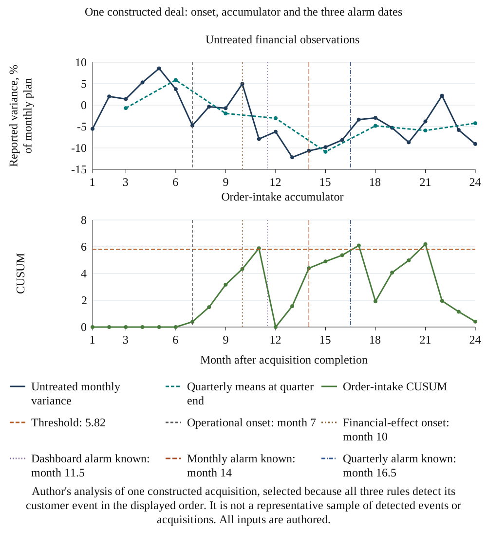
Figure 1 follows one constructed deal with a single customer event. The onset is in month 7 and reported variance is expected to begin moving in month 10, three months later. The order-intake accumulator crosses its threshold and the dashboard alarm becomes known in month 11.5. The monthly accounts alarm becomes known in month 14.0 and the quarterly report alarm in month 16.5.
Scroll horizontally to read the figure at full size. You can also open the full-size figure.
Author's analysis of one constructed acquisition, selected because all three rules detect its customer event in the displayed order. It is not a representative sample of detected events or acquisitions. All inputs are authored.
This selected path shows the separation between operational onset, financial observation and alarm availability. The reported monthly series contains noise; quarterly averaging changes the size and timing of an observation; the accumulator collects persistent adverse deviations and resets at a crossing. The displayed example was chosen because all three regimes detected the customer event in the stated order. It supplies no evidence about a typical real acquisition or an unconditional ranking of monitoring rules.
12 Single-indicator performance
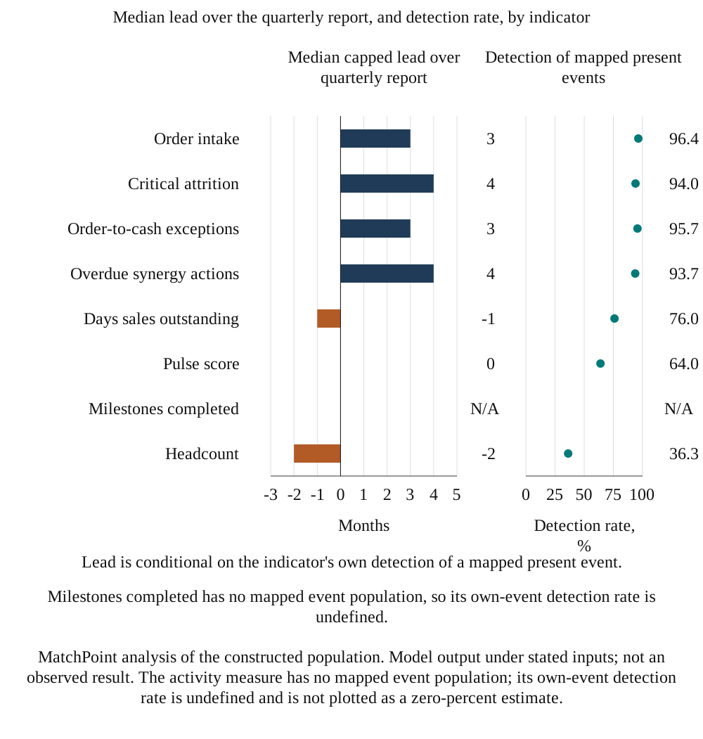
Table 7 evaluates each indicator separately at a 10 per cent single-indicator horizon target. Detection is the first post-onset alarm for a channel the indicator points to. Delay runs from onset to alarm availability. The displayed lead subtracts indicator availability from quarterly-alarm availability. When quarterly detection is absent, its time is replaced by the horizon plus its reporting lag. These are finite-horizon, model-defined summaries; the replacement can make indicator lead look larger than a comparison restricted to mutually detected events.
| Indicator | Role | Detection of own events | Median delay from onset (months) | Median lead over quarterly (months) | Earlier than quarterly | False alarms per deal-year |
|---|---|---|---|---|---|---|
| Order intake | Informative | 96.4% | 3.5 | 3.0 | 73.8% | 0.042 |
| Critical attrition | Informative | 94.0% | 4.5 | 4.0 | 71.5% | 0.043 |
| Order-to-cash exceptions | Informative | 95.7% | 4.5 | 3.0 | 70.2% | 0.039 |
| Overdue synergy actions | Informative | 93.7% | 4.5 | 4.0 | 75.0% | 0.041 |
| Days sales outstanding | Informative, delayed | 76.0% | 7.5 | -1.0 | 38.7% | 0.034 |
| Pulse score | Weak | 64.0% | 7.5 | 0.0 | 45.9% | 0.084 |
| Milestones completed | Activity measure | No mapped events | n/a | n/a | n/a | 0.052 |
| Headcount | Weak, delayed | 36.3% | 9.5 | -2.0 | 34.3% | 0.043 |
MatchPoint analysis of the constructed population. Model output under stated inputs; not an observed result. Lead is censored at the end of the horizon for events the quarterly rule does not detect.
The four direct indicators detect the large majority of their own events within the horizon at the single-indicator budget and lead the quarterly report at the median by the margins in Table 7. Days sales outstanding, which moves two months after onset, has a negative displayed median lead over the quarterly report. The pulse score detects fewer events and has the highest false-alarm rate of the eight, and headcount, which moves three months after onset, is two months behind. The activity measure never detects an event and returns a net value of -1.05 per deal, because every alarm it raises is a false one.
Figure 2 presents the same results graphically. The bars measure the median lead over the quarterly report and the markers the detection rate, so an indicator that leads but detects few events is distinguished from one that detects most events but late. The four direct indicators combine a high detection rate with a positive lead. Days sales outstanding and headcount combine a lower detection rate with a negative lead, and the activity measure appears with no detection at all.
Scroll horizontally to read the figure at full size. You can also open the full-size figure.
MatchPoint analysis of the constructed population. Model output under stated inputs; not an observed result. The activity measure has no mapped event population; its own-event detection rate is undefined and is not plotted as a zero-percent estimate.
The result distinguishes timing from channel coverage in this constructed population. Days sales outstanding has the largest single-indicator net value, 10.81, under its two-channel mapping, while order intake returns 10.76 and critical attrition 4.46. Those rankings depend on the authored channel severities, incidence, noise and response model. Section 17 examines sampling variation within the same population. It does not establish a real-world preference order for these metrics.
13 Recovery against quarterly reporting, monthly accounts and perfect information
Table 8 compares the regimes on the test population. Without action, leakage over 24 months averages 77.7 percentage points of one month of plan per deal. The oracle, which acts one month after each onset, reduces it to 31.1, so the avoidable amount is 46.6. The quarterly report recovers 56.8% of that amount, monthly accounts 65.8% and the dashboard of 5 indicators 74.2%.
In the constructed population there are 20,081 present channel events. The dashboard detects 18,908 of them within the generated horizon. The monthly rule does not detect 433 of those dashboard-detected events, and the quarterly rule does not detect 511. The detected sets are therefore non-nested. Marginal event detection is 94.2% for the dashboard, 97.2% for monthly accounts and 96.8% for quarterly reporting. Among each regime's detected events, median onset-to-availability delays are 4.5, 6.0 and 7.5 months respectively. These conditional timing summaries compare different detected subsets and establish no real-world coverage limit.
In Equation 4a, m_{L,0} is mean accumulated leakage with no action, m_{L,r} is mean accumulated leakage under regime r and m_{N,r} is its mean count of false-labelled investigations. These are arithmetic means across the finite test population. The charge c is 10 percentage points of one month of plan per false investigation. Equation 4b divides avoided leakage by the amount avoided by the perfect-information reference. That ratio is defined here because the reference denominator is positive.
| Regime | Leakage (% of a month's plan) | Leakage avoided | Share of avoidable leakage recovered | False alarms per deal | Net value | Basis |
|---|---|---|---|---|---|---|
| No action (reference) | 77.68 | 0.00 | 0.0% | 0.000 | 0.00 | Leakage runs its course |
| Quarterly report | 51.20 | 26.48 | 56.8% | 0.144 | 25.04 | Eight tests, 1.5-month lag |
| Monthly accounts | 47.01 | 30.67 | 65.8% | 0.130 | 29.37 | CUSUM, 1-month lag |
| Dashboard of 5 indicators | 43.11 | 34.57 | 74.2% | 0.221 | 32.36 | Budgeted thresholds |
| All eight, unbudgeted | 40.29 | 37.39 | 80.2% | 0.757 | 29.83 | Each at its own 10% budget |
| Full-information response benchmark | 31.07 | 46.61 | 100.0% | 0.000 | 46.61 | Known latent onset; same authored response efficacy |
MatchPoint analysis of the constructed population. Model output under stated inputs; not an observed result. Units: percentage points of one month of plan per deal, over 24 months.
After false-investigation costs, the dashboard returns 32.36 units per acquisition, 7.32 above quarterly reporting and 2.99 above monthly accounts. Units are percentage points of one month of plan, accumulated over 24 months. The gap from this selected rule to the perfect-information benchmark is 14.25. It is headroom relative to this rule under the model; a different rule or response could capture a different amount. The unbudgeted eight-indicator dashboard recovers 80.2% and generates 0.757 false alarms per acquisition, compared with 0.221 for the selected dashboard. Their break-even false-investigation cost is 5.3 units.
The quarterly-to-monthly reporting change produces the larger gain in this base experiment. Among dashboard-detected model events, the displayed finite-horizon median lead is 3.0 months over quarterly reporting and 1.5 over monthly accounts. The dashboard is earlier than the quarterly rule for 69% of its detected events. For 31% of dashboard-detected events, alarm availability is at or before the first model month of financial effect. Equality is included in this last measure, and no universal pre-loss detection rate is inferred.
The extra-cost sensitivity in Table 9 adds an authored charge for each true-labelled investigation while leaving the signal paths, response rules and false-investigation charge unchanged. It exposes a cost excluded from the primary score. It does not measure staff capacity, a real response budget or the value of suppressing repeat investigations after a successful action.
| Extra cost per true-labelled investigation | Quarterly net | Monthly net | Dashboard net | Unbudgeted eight-indicator net | Dashboard minus monthly |
|---|---|---|---|---|---|
| 0 | 25.04 | 29.37 | 32.36 | 29.83 | 2.99 |
| 0.25 | 24.48 | 28.59 | 31.69 | 28.96 | 3.10 |
| 1 | 22.78 | 26.25 | 29.67 | 26.35 | 3.42 |
| 2 | 20.51 | 23.12 | 26.98 | 22.87 | 3.86 |
Authored extra cost in percentage points of one month of plan per investigation. Model paths and responses remain frozen. No cost is an observed transaction estimate.
The additional-cost sensitivity changes the primary comparison in a specific direction. With no extra charge for true-labelled investigations, dashboard net value is 32.36 units and monthly-accounts net value is 29.37, a difference of 2.99. At an extra cost of two units per true-labelled investigation, their net values become 26.98 and 23.12 and the difference becomes 3.86. This occurs because the monthly rule generates a mean of 3.125 true-labelled alarms per acquisition, compared with 2.693 for the selected dashboard. The same charge therefore subtracts more from monthly accounts. These are workload properties of frozen constructed paths; the calculation measures no actual staff saving or implementation return.
Repeated alerts also raise a question about the unit being costed. The experiment charges each recorded alarm under its stated classification. A practical team could combine several alerts into one investigation episode or require a fresh investigation after a materially different observation. Successful corrective action could also change subsequent operating signals, an effect excluded from the frozen-signal model. Record the alert, the investigation episode and the response separately before estimating a real cost. A low cost per alert can coexist with a high cost per resolved issue when many alerts concern the same underlying cause. The current results evaluate none of those alternative workflow policies.
The practical evaluation should also test whether investigation capacity changes response timing. The model uses a fixed response delay and contains no queue of cases competing for the same managers, specialists or operating resources. Consequently a higher alarm count does not extend its assumed response time. In a proposed live evaluation, retain the dates of assignment, investigation, approval and implementation, with unresolved cases still in the record. Examine the relationship between workload and elapsed response time before assuming the model's fixed delay is feasible. The warning's economic contribution depends on whether an authorised operating response can occur before the relevant loss becomes difficult to recover.
These limits matter when a board allocates a monitoring budget. The expenditure request should distinguish building the data feed, maintaining definitions, investigating signals and delivering the proposed response. Identify which cost is recurring, which is conditional on an alarm and which belongs to a wider integration initiative that would occur anyway. The simulation's ten-unit false-investigation charge and the separate true-investigation sensitivity are authored comparison inputs. They provide no evidence of a reasonable fee, staffing allocation or cost ratio for an acquirer. Replace them with documented costs or show explicitly conditional ranges before using a comparison in a spending decision.
A useful pilot decision can therefore be narrow. Specify the exposure to be monitored, the existing information comparator, the permitted records and the response decision that an earlier warning could change. Set a review date and record what evidence would justify continuation, revision or retirement. Keep mandatory operating controls active throughout. The initial output can establish data availability and investigation workload even when the period is too short to estimate protected financial value. That limited result is useful for the next resource decision. It should retain its actual evidential scope when the team reports progress to the board.
14 Dashboard composition and the investigation budget
Table 10 builds the dashboard greedily on a separate selection pool of 6,000 deals: at each size, the added indicator maximises the evaluated net value, and the thresholds target a 25 per cent dashboard horizon false-alarm probability. The first indicator chosen, days sales outstanding, receives the whole 25 per cent target when evaluated alone and points to two channels. Its threshold differs from the 10 per cent standalone test in Table 7. Its selection reflects the joint effect of coverage, timing, thresholds and authored costs. It supplies no universal adoption order. The published rule is selected on one pool and reported on a separate test pool.
| Indicators | Added indicator | Per-indicator budget | Threshold h (sd) | Share of model-avoidable leakage recovered | False alarms per deal | Net value |
|---|---|---|---|---|---|---|
| 1 | Days sales outstanding | 25.0% | 3.45 | 31.6% | 0.188 | 12.84 |
| 2 | Overdue synergy actions | 13.4% | 4.47 | 50.3% | 0.208 | 21.35 |
| 3 | Order intake | 9.1% | 5.10 | 59.6% | 0.210 | 25.66 |
| 4 | Critical attrition | 6.9% | 5.49 | 68.4% | 0.217 | 29.70 |
| 5 | Order-to-cash exceptions | 5.6% | 5.82 | 74.2% | 0.221 | 32.36 |
| 6 | Headcount | 4.7% | 6.06 | 72.9% | 0.227 | 31.71 |
| 7 | Milestones completed | 4.0% | 6.29 | 71.5% | 0.238 | 30.94 |
| 8 | Pulse score | 3.5% | 6.52 | 70.7% | 0.281 | 30.15 |
MatchPoint analysis of the constructed population. Model output under stated inputs; not an observed result. Net value is in percentage points of one month of plan per deal.
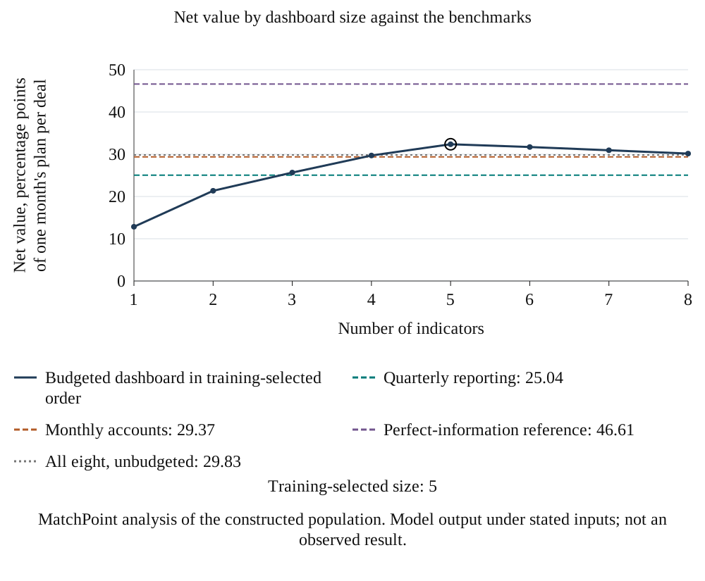
Net value rises to 32.36 at 5 indicators and then falls. By size eight it is 30.15, because each added indicator tightens every threshold through the family budget while contributing little detection. The five indicators chosen are days sales outstanding, overdue synergy actions, order intake, critical attrition, order-to-cash exceptions. Choice matters as much as number: across all 56 possible dashboards of 5 indicators the net value ranges from 10.21 to 32.36, with a mean of 22.17, so a randomly chosen set of the same size is worth far less than the selected one.
Figure 3 compares the selected dashboard at each size with quarterly reporting, monthly accounts, the perfect-information reference and the unbudgeted candidate set. Every budgeted size targets the same horizon false-alarm probability. This controls one statistical quantity; it does not measure available investigation capacity. Repeated-alarm counts, triage effort and corrective-action cost require separate evaluation. The best size on the held-out test population is 5, reported as a diagnostic; the published dashboard remains the one chosen on the selection population.
Scroll horizontally to read the figure at full size. You can also open the full-size figure.
MatchPoint analysis of the constructed population. Model output under stated inputs; not an observed result.
The experiment identifies a cost of admitting weak or late indicators when the family probability target is held fixed. Additional indicators tighten the other thresholds and can add little useful channel coverage. A real admission decision should specify the incremental exposure covered, the information date, shared dependence with existing metrics and expected investigation burden. The simulated optimum of 5 indicators applies only to this candidate set, selection procedure and authored population.
15 Signal strength and financial-effect timing
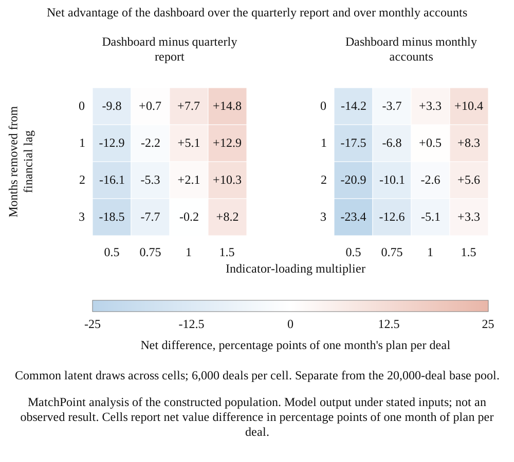
The dashboard's lead is an authored property, so Figure 4 varies signal strength and financial-effect timing. The horizontal axis multiplies every indicator loading. The vertical axis removes months from each financial lag, with a zero floor. Every cell reports net value of the frozen dashboard minus its comparator for 6,000 constructed acquisitions. The cells reuse seed 44 and common latent and noise draws, with thresholds held at their base values. This sensitivity population is separate from the 20,000-acquisition base test pool.
Scroll horizontally to read the figure at full size. You can also open the full-size figure.
MatchPoint analysis of the constructed population. Model output under stated inputs; not an observed result. Cells report net value difference in percentage points of one month of plan per deal.
Against the quarterly report, the base cell is 7.7; at 0.75 of base strength it falls to 0.7, and at half strength to -9.8. Against monthly accounts the base cell is 3.3, but it turns negative, to -3.7, at 0.75 of base strength, and removing three months from the financial lag at base strength gives -5.1. The dashboard also loses to the quarterly report in the corner where indicators are half as strong and financial effects arrive three months sooner, at -18.5.
The map locates the condition under which the investment in leading indicators is justified. At base strength or below, where the financial series reacts within a month or two of the cause, or where indicators carry weak signal, monthly accounts alone match or beat the dashboard. Only where the indicators are sharp does the dashboard win against both comparators across the map: at 1.5 times base strength it wins by 8.2 and 3.3 even with a three-month shorter lag. The edge over monthly accounts is therefore small and conditional, not robust.
16 Stress tests with frozen thresholds
Table 11 applies five stresses to the test population while holding the dashboard set, thresholds and benchmark rules fixed at their base values. The diagnostic columns report the share of leakage-free deals with a dashboard alarm, the share of leakage deals found by the accounts only and the alarm rate of the activity measure assigned zero event loadings in this experiment. These are model diagnostic signatures; their usefulness for recognising an actual failure requires transaction-specific evaluation.
These cases should be read as a checklist of how a dashboard fails. Noise, management of indicators and definition breaks damage the dashboard through different mechanisms and leave different traces, and none of them is visible in the headline recovery share alone: the noisy case recovers slightly more than the base case while its net advantage over monthly accounts becomes strongly negative. A board that tracks only how much leakage its alarms preceded would therefore reward the worst-behaved dashboard.
| Case | Dashboard recovered | Quarterly recovered | Monthly accounts recovered | Dashboard net advantage over monthly accounts | Leakage-free deals with a dashboard alarm | Leakage deals found by accounts only | Activity-measure alarm rate |
|---|---|---|---|---|---|---|---|
| Base | 74.2% | 56.8% | 65.8% | 2.99 | 24.9% | 2.9% | 5.8% |
| Noisier indicators | 74.8% | 56.8% | 65.8% | -12.04 | 88.2% | 4.1% | 35.0% |
| Faster accounts | 74.2% | 64.1% | 69.4% | 1.34 | 24.9% | 2.9% | 5.8% |
| Shorter financial lag | 66.4% | 61.4% | 70.1% | -2.92 | 24.9% | 3.3% | 5.8% |
| Managed indicators | 56.1% | 56.8% | 65.8% | -5.44 | 24.9% | 17.5% | 5.8% |
| Definition break | 77.6% | 56.8% | 65.8% | -10.86 | 39.7% | 2.4% | 24.2% |
MatchPoint analysis of the constructed population. Model output under stated inputs; not an observed result. Net advantage in percentage points of one month of plan per deal.
When indicator noise rises, the dashboard recovers about the same share, 75%, but 88% of leakage-free deals now produce an alarm against 25% in the base case and the net advantage over monthly accounts turns negative. The signature is a rise in alarms with no change in the accounts. When managers manage three indicators, the dashboard recovered share falls to 56%, below the quarterly report in the same case, and the share of leaky deals found only by the accounts rises to 17%: the dashboard is quiet while the financials move.
A definition break, here a system change that shifts every indicator at month 9 in one deal in five, raises the dashboard false-alarm rate to 40% and the alarm rate of the activity measure to 24% from 6%. The model dates the break by construction; a real analyst would look for alarms across unrelated indicators in the same month. With financial effects two months sooner, monthly accounts recover 70% against the dashboard's 66% and the quarterly report's 61%. With faster accounts, the quarterly report recovers 64%, monthly accounts 69% and the dashboard 74%. In both cases a dashboard that was justified at the base lags needs re-testing.
17 Repeated samples from the constructed population
Table 12 describes 1,000 repeated samples of each stated size drawn with replacement from the fixed constructed test population. Each sample ranks single indicators by net value. The columns show agreement with that finite population's best indicator and best four, model regret from the selected top indicator and the frequency with which the sampled dashboard advantage is negative. These samples reuse a known authored population; they do not reproduce variation in definitions, sectors, acquirers, cohort access or observed intervention decisions.
| Completed deals | Expected events | Reference-best indicator ranked first | Reference-best four identified | Mean regret of top pick | Dashboard minus monthly accounts, 5th to 95th | Samples with negative dashboard-minus-monthly net | Samples with negative dashboard-minus-quarterly net |
|---|---|---|---|---|---|---|---|
| 30 | 30 | 29% | 67% | 0.67 | -1.5 to 7.4 | 12% | 1% |
| 60 | 60 | 34% | 81% | 0.44 | 0.1 to 6.0 | 4% | 0% |
| 120 | 120 | 37% | 95% | 0.36 | 0.8 to 5.2 | 1% | 0% |
| 240 | 240 | 38% | 98% | 0.26 | 1.4 to 4.5 | 0% | 0% |
| 480 | 480 | 43% | 100% | 0.20 | 1.9 to 4.1 | 0% | 0% |
| 960 | 960 | 50% | 100% | 0.11 | 2.2 to 3.8 | 0% | 0% |
MatchPoint analysis of the constructed population. Model output under stated inputs; not an observed result. Cohort sizes equal expected events because the model has one event per deal on average. Selection and confounding in real cohorts are not represented.
In 12% of simulated samples of 30 acquisitions, the dashboard-minus-monthly estimate is negative, falling to 1% at 120 deals. The true best single indicator, days sales outstanding, is ranked first in only 37% of studies of 120 deals and 50% at 960, because order intake is almost level with it, while the best four, order intake, order-to-cash exceptions, overdue synergy actions, days sales outstanding, are identified as a set in 95% at 120 deals. The 5th to 95th percentile range of the dashboard's net advantage over monthly accounts is -1.5 to 7.4 at 30 deals and 0.8 to 5.2 at 120.
The simulated uncertainty falls with sample size. The dashboard-minus-monthly interval is -1.5 to 7.4 at 30 sampled acquisitions and 0.8 to 5.2 at 120. Mean regret from the sample's top single indicator is 0.67, 0.36 and 0.11 at 30, 120 and 960. These are repeated-sampling summaries for the experiment. An acquirer should not use them to decide that it has enough actual transactions or that a specific metric can be safely dropped.
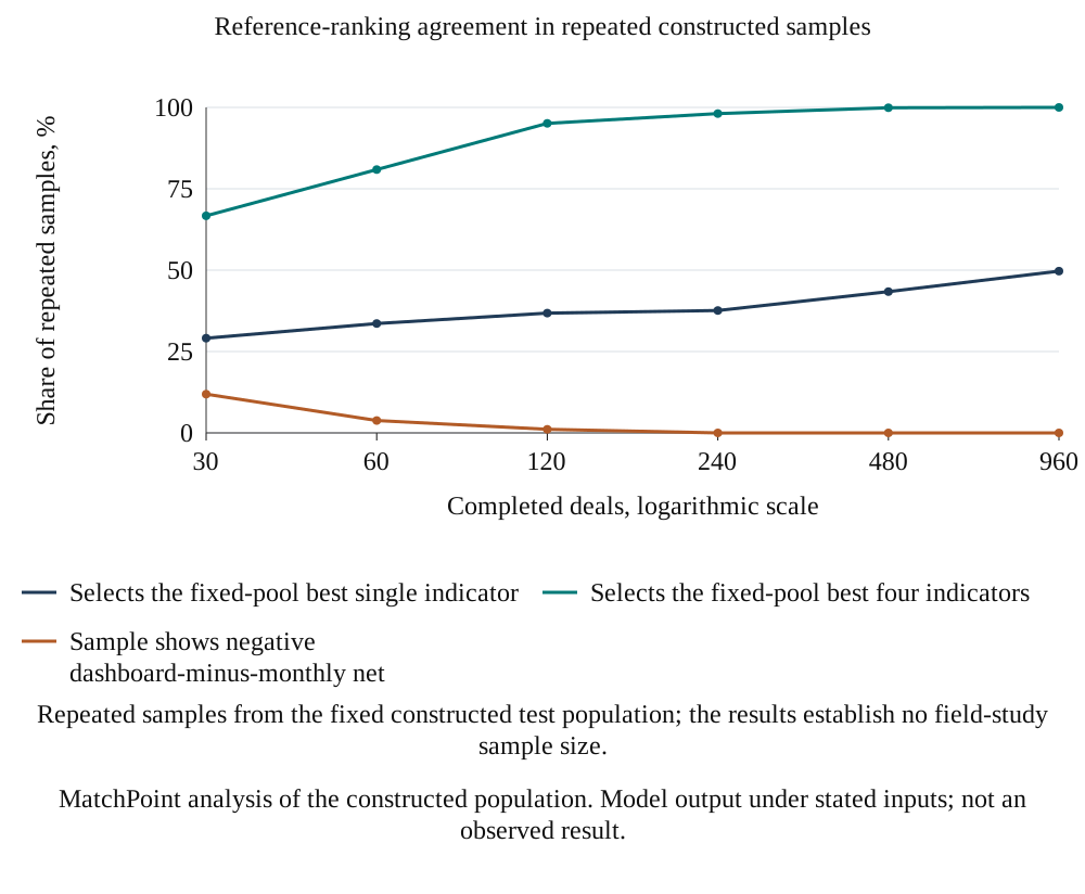
Scroll horizontally to read the figure at full size. You can also open the full-size figure.
MatchPoint analysis of the constructed population. Model output under stated inputs; not an observed result.
Figure 5 visualises the same repeated samples. A real sample-size design must specify its event rate, minimum decision-relevant difference, clustering by acquirer, follow-up, missingness, measurement error and evaluation method. None of those real-world quantities is estimated here. A real cohort could be more or less informative than a sample from this population, so the displayed intervals are not a mathematical lower bound on empirical uncertainty.
18 Intervention changes the outcome recorded after an alarm
A response can change the financial outcome subsequently recorded after an alarm. Lenert, Matheny and Walsh discuss this feedback problem for clinical prognostic models. [9] That setting supports a methodological caution about evaluation after intervention; it supplies no acquisition-specific response effect. The experiment compares two generated financial paths using identical event and noise draws, with and without the model response. Its randomised withholding calculation is an arithmetic demonstration within the simulation.
In Equation 5a, M^(0) indicates a reported quarterly miss in the 12 months after the first dashboard alarm becomes available when no response is applied. Here A=1 denotes an alarmed acquisition with that complete reporting-availability follow-up observable within the generated horizon; the equation refers to this eligible cohort. There are 8922 eligible acquisitions and 5924 late alarms excluded from the primary comparison. In Equation 5b, H_j is the jth acquisition in a nonempty, randomly selected eligible no-response subset H, and n_H is the number selected. The estimator averages their no-response miss outcomes. A real acquirer cannot observe both response states for the same event; the calculation supplies no authority to withhold a protective action.
| Measurement | Reported-miss share under stated cohort/window | Reading |
|---|---|---|
| Eligible alarms: no action (constructed reference) | 87.6% | Complete 12-month known-date follow-up; eligible cohort |
| Eligible alarms: latent-triage response policy | 70.8% | Same eligible cohort and noise; action changes leakage only |
| Holdout of 25% of 60 alarmed deals | 87.8% (5th to 95th: 71% to 100%) | Constructed repeated-sampling estimate on eligible complete-window alarms |
| No alarm over 24 months: first-four-quarter outcome | 14.3% | Different descriptive cohort/window; not a PPV comparator |
Constructed complete-follow-up comparison. A miss is a quarterly report available in the 12 months after the first alarm becomes known, with variance below minus 5% of plan. Late alarms are excluded from the primary cohort; the no-alarm row has a separate first-four-quarter window.
Among the eligible alarmed acquisitions, the reported-miss share is 88% without response and 71% with response. The corresponding shares without a later reported miss are 12% and 29%. In repeated simulated groups of 60 eligible alarmed acquisitions, a 25 per cent no-response allocation estimates 88% on average with a 5th-to-95th range of 71% to 100%. These outputs concern constructed paths and a complete-follow-up subset, not observed accuracy or the effect of a real intervention. In total, 14846 acquisitions alarmed. The complete-follow-up restriction selects an earlier-alarm group; its reported shares should not be transferred to all alarms.
For the correctly channel-matched first-alarm subgroup, the model reported-miss share changes from 97% to 78% after response. The separately described no-dashboard-alarm cohort has a 14% miss share in its first four financial quarters; its population and window differ from the alarmed comparison. Late alarms excluded from the complete-follow-up comparison remain recorded in the diagnostic output. Every empirical assessment should preserve these cohort and follow-up distinctions.
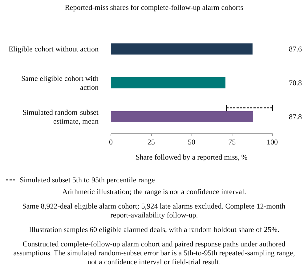
Scroll horizontally to read the figure at full size. You can also open the full-size figure.
Constructed complete-follow-up alarm cohort and paired response paths under authored assumptions. The simulated random-subset error bar is a 5th-to-95th repeated-sampling range, not a confidence interval or field-trial result.
19 A feasible transaction-evaluation protocol
The proposed real study begins with lawful access and a measurement agreement. Define the participating acquirers, the acquisitions eligible for inclusion, the observation period and the records available on each decision date. Include acquisitions with no recorded leakage and document exclusions, incomplete histories and changes of ownership. The unit of analysis can be the acquisition-month, with event and channel records linked to it. Repeated observations from one acquisition or one acquirer need appropriate dependence treatment. No access to such a cohort has been established for this paper.
Preserve two dates for each record: when the underlying event occurred and when the information became available to the authorised decision-maker. Define the outcome and materiality rule before examining indicator performance. Save the original approved plan and every subsequent reforecast. Keep the raw alarm, the human investigation, the adjudicated event and the action as separate records. Agreement between an alarm and an outcome after the fact can reflect common causes, outcome-informed classification or intervention. The evaluation method should address those possibilities explicitly.
Processing customer and workforce records requires the applicable legal basis, permissions, purpose limitations, retention rules and security measures. The UAE federal regime contains consent requirements and specified exceptions; the applicable law and any relevant sector or free-zone regime must be checked for the actual processing. [11] Aggregate role-level reporting can reduce personal detail, but aggregation alone does not establish compliance. Obtain advice for the relevant controller, jurisdictions, transfers and data uses before accessing or combining records.
A practical first stage is shadow evaluation: apply frozen candidate rules to lawfully available records, log their signals and measure their workload alongside existing management controls. Shadow operation must not suppress information or delay an action that safety, law, contract or ordinary risk management already requires. A prospective experiment on an incremental, discretionary intervention would need genuine uncertainty about its value, a lawful and ethically acceptable protocol, appropriate approvals and stop rules. Where experimentation is unavailable, use documented intervention records and a transparent observational method with its remaining confounding limitations.
| Element | Requirement | Reason |
|---|---|---|
| Unit | Acquisition-month linked to event and channel records | Preserves time and dependence structure |
| Cohort | Document all eligible acquisitions, exclusions and missing histories | Exposes selection and incomplete outcomes |
| Timestamps | Event, available-at, alarm, response and reported outcome | Limits hindsight and measures decision delay |
| Definitions | Frozen populations, thresholds and versioned changes | Supports reproducible comparisons |
| Evaluation | Shadow testing; observational limitations; experiments only with genuine equipoise and approvals | Preserves protective action and exposes intervention effects |
| Privacy | Applicable legal basis, access, transfers, retention and safeguards [11] | Requires transaction-specific legal review |
| Sample design | Estimate event rate, clustering, missingness and decision-relevant difference | No empirical minimum is established here |
| Analysis plan | Pre-specified comparators, outcomes, follow-up and sensitivity tests | Limits selective interpretation |
MatchPoint proposed design. Entries are requirements, not findings; none has been implemented.
20 The board pack and its decision record
A board pack on integration leakage should state, for each channel, the indicator, its threshold, the date it last crossed and the date the response began. It should report investigation counts and repeated-alarm workload against a separately specified capacity and cost plan, the share of alarms investigated and the evidence for any suppression. The horizon false-alarm probability target should be assessed on a stated leakage-free evaluation cohort with its denominator and horizon. These records help the board investigate whether a quiet dashboard reflects healthy integration, managed indicators, changed definitions or threshold drift.
The pack should show the indicator's lead over the financial comparator on past events, including its range, detection denominator and finite-follow-up convention. It should separately show the estimated horizon false-alarm probability against its stated target and repeated investigation counts against a capacity and cost plan. The shortfall to plan should appear beside indicator readings so that divergence is visible. The model's gaming case illustrates one authored mechanism that creates such a divergence.
The proposed pack in Table 15 places the operational readings beside the accounting and cash record, with unresolved items, population sizes and uncertainty visible. A divergence can prompt investigation of a business issue or of the measurement system. The pack should also show changes to definitions, suppression decisions and the last evaluation period. Threshold crossing, completed action, accounting recognition and realised cash are separate states with separate evidence.
| Item | Content | Question answered |
|---|---|---|
| Channel panel | Indicator, threshold, last crossing, response date | Which channels are alarming and since when |
| Probability and workload panel | Horizon false-alarm probability versus target on a defined evaluation cohort; repeated investigation counts versus a separate capacity and cost plan | Whether probability calibration and investigation workload remain acceptable under the stated definitions |
| Divergence panel | Indicators beside monthly variance to plan | Whether the dashboard and the accounts agree |
| Lead record | Past lead over financial series, with range | Whether the dashboard still earns its place |
| Change log | Definition and system changes | Whether a simultaneous alarm is a break |
| Intervention record | Alarm, actual response, obligation and subsequent outcome | What action changed the observable outcome |
MatchPoint proposed layout. Entries describe information to show; they are not findings.
21 AI-assisted collection and indicator evaluation
Contract, invoice and workstream-note extraction are candidate uses for automation in assembling an indicator. Their accuracy, coverage, security, maintenance effort and cost require measurement on the documents and operating context in use. This paper tests no trained extraction system and establishes no cost saving. Its model concerns the value of an available signal under stated loadings and timing. Adding an AI score would require an explicit mechanism, a frozen input version and comparison with the existing information and decision process.
Evaluation should name the decision under study and preserve the same financial comparator, information dates and outcome definition across candidate tools. Report missing fields, abstentions, extraction errors and manual-review effort alongside performance. A tool that changes which records are available changes the evaluation population. A tool whose output triggers action also changes later outcomes, creating the intervention issue discussed in [9]. Each of those effects needs a stated analysis rather than an assumed accuracy or uplift.
An automated tool is also exposed to definition breaks and management failures. A system reading contracts or tickets can change its output when the source system, language or extraction rule changes, so its version and inputs should be retained. Evaluate any proposed indicator against its defined mechanism, coverage, accuracy, timeliness and total review and maintenance cost. This paper establishes no reduction in collection cost and supplies no validated AI-derived indicator.
22 Applying the framework to a transaction
A transaction team can begin by mapping the approved acquisition case to the customer, capability, operations and benefit exposures it actually contains. Assign source records and owners to each exposure. State when a potential deterioration would be reflected in existing management information and what additional decision a proposed warning could support. Treat the model's candidate indicators as examples with authored loadings. Their inclusion in this experiment establishes no empirical suitability for a transaction.
Next, define the adverse direction, population, available-at date and version for each candidate. Calibrate on an appropriate baseline and evaluate on separate later records or acquisitions. Set an explicit tolerance for false-alarm probability and a separate investigation-capacity plan, including repeated signals. Report indicators alongside the monthly accounting and cash record, retain responses and suppressions, and investigate missingness or definition changes. Any revised rule should have its own version and independent evaluation period.
The proposed tools below make these requirements operational. They do not prescribe the same thresholds, timing or legal arrangements for every sector or jurisdiction. An acquirer should adopt only the parts it can support with its value case, actual records, delegated authorities and applicable obligations.
23 Reproducibility and internal controls
The scientific run uses fixed seeds for calibration, selection, testing, the sensitivity map and repeated samples. It checks 74 internal identities, calibration tolerances and stated directional properties. Separate records retain the exact source, model code, unrounded diagnostic arrays and rendered exhibit inputs. Internal reconciliation establishes what the program calculated for this version; it does not establish that the authored event relationships or response rates describe acquisitions.
Table 16 summarises the internal controls. The no-response reference has zero recovered share and the perfect-information reference has share one by the chosen denominator. Under the base financial lags the latter removes the model's 60 per cent fraction before financial losses begin, making its residual leakage mechanically 40 per cent of baseline. These identities help identify implementation errors. Their satisfaction supplies no independent evidence for the assumptions that created them.
| Control | Result |
|---|---|
| Asserted identities and directional checks | 74 passed |
| Calibration of accumulators and quarterly line | False-alarm probability within tolerance of the 25% budget |
| Budget splitting | Sidak identity holds exactly |
| Oracle and no-action shares | One and zero |
| Per-deal and aggregate net value | Reconcile |
| Random no-response subset in simulation | Repeated Monte Carlo estimate within stated tolerance |
| Stress directions | Each asserted |
| Pools and seeds | Fixed; test pool 20,000 deals |
MatchPoint model controls. Counts are from the model run reported in this paper.
The controls establish that the code is internally consistent. They do not establish that the premise holds. Outcomes are generated from the same events the indicators read, so the experiment shows how detection rules behave when indicators lead by the authored margin; it does not show that real indicators do.
24 Build the warning record before Day One
A warning system needs a stable starting record. Before completion, the integration lead should identify the value assumptions that the acquisition committee actually approved: the customer relationships to retain, the capabilities on which delivery depends, the operating changes to make and the cash that each planned benefit is expected to release. Each assumption should have an evidence source, an accountable owner and an expected date. A revenue forecast without a corresponding customer population cannot support a customer-retention indicator. A synergy estimate without a dated action cannot support an overdue-action measure. These are proposed requirements for using the framework, rather than observations about any acquirer's current practice.
Legal restrictions on pre-completion information sharing remain applicable. A team should establish the permitted aggregate measures and any clean-team arrangements with its advisers before transferring competitively sensitive or personal information. When a usable baseline is unavailable at completion, the board should see that limitation in the first pack. It should receive the raw counts and the period covered while the team establishes a baseline, with thresholds treated as provisional. Assigning a precise standard-deviation score to a short or incompatible history would give the score an authority that its inputs do not support.
The proposed timeline in Table 17 separates preparation, initial observation and later evaluation. The dates are management design choices for a transaction team to adapt. They are unrelated to a statutory reporting deadline. The Day-One objective is continuity of observation and decision ownership. Testing an indicator's predictive performance requires later outcomes, so a Day-One dashboard can be operationally available while its predictive value remains unestablished. Keeping those states separate lets the board use a critical customer exception immediately and reserve judgement about the statistical model.
| Stage | Required work | Evidence for the board |
|---|---|---|
| Before completion | Map the approved value case to permitted source records; appoint owners; preserve baseline definitions | Versioned value case and list of data gaps |
| Day One | Confirm access, owners and continuity of customer, people and operating records | Availability register with explicit missing fields |
| First two weeks | Reconcile populations and accounting mappings; log alarms and responses separately | Definition changes and unresolved reconciliation items |
| First monthly close | Compare operational signals with actual accounts and cash; keep provisional thresholds identified | Matched reporting dates and contribution bridge |
| End of first quarter | Review alarm workload, missingness and adjudicated event records | Investigation history and evidence for any threshold change |
| Subsequent review | Evaluate the frozen rules on later deals or periods and review sector transferability | Out-of-time results, limitations and change decision |
Author-proposed sequence. Timing must be adapted to the deal, information-sharing restrictions and actual reporting capability.
The acquisition case should remain retrievable after budgets are revised. Otherwise an integration team can improve apparent performance by changing the comparator. Keep the original approved case, a dated operating reforecast and reported actuals as separate records. A board may legitimately approve a changed plan after new information arrives. The record should then show the reason and the effect on the expected benefit, so that a favourable reforecast variance does not erase a shortfall against the acquisition decision. This discipline also helps distinguish a purchase-accounting adjustment from a change in operating delivery.
25 Give every alarm an owner and an escalation decision
An alert requires a named person who can investigate its underlying record and a person who can authorise a response. The model assumes that an alarm reaches the correct leakage channel and that a response becomes effective after a fixed delay. A real organisation has to create those links. For example, an order-intake warning may involve an account director, a pricing decision and a delivery constraint. Routing the score only to the integration office can add a hand-off before any of those people acts. The response date should therefore be measured from the information's availability, through investigation and approval, to the actual operating change.
Table 18 gives a proposed RACI for that process. Accountable means the single role answerable for the decision; responsible means the role performing the work; consulted and informed describe the other participants. The table uses role titles so a team can adapt it without implying that a particular corporate structure is required. The chief financial officer owns reconciliation with the approved financial case. Operational owners retain responsibility for customer and service decisions within their authority. Legal, compliance and data-protection specialists determine the applicable constraints on a proposed action or use of records.
| Activity | Accountable | Responsible | Consulted or informed |
|---|---|---|---|
| Define the financial baseline and benefit measure | CFO | Finance controller | Integration lead and business owner consulted |
| Maintain indicator definitions and available-at dates | Integration lead | Data or workstream owner | Finance and data-protection specialists consulted |
| Investigate an operational warning | Business owner | Named workstream lead | Integration office and finance consulted |
| Approve a material response or spending request | Holder of the relevant delegated authority | Business owner preparing the decision | CFO, legal and compliance consulted as applicable |
| Reconcile claimed benefit with cash and accounts | CFO | Finance controller | Workstream owner consulted; integration lead informed |
| Change a threshold or retire an indicator | Designated risk or integration committee | Analyst and integration lead | Business owner and independent reviewer consulted |
Author-proposed allocation. RACI means responsible, accountable, consulted and informed; actual delegations and reserved matters govern.
Escalation should depend on potential consequence, contractual obligations and available response time. A statistical threshold cannot replace an existing safety, regulatory or critical-customer escalation. Those cases should follow the established protective process as soon as the relevant facts are known. For ordinary operating warnings, the decision record should state what was checked, what remained uncertain, the action selected and when the owner expects new evidence. A team can choose different investigation deadlines for different risks. This paper supplies no empirically validated deadline and no universal materiality percentage.
Suppressions need a reason and an expiry or review date. A known data migration may explain why several indicators move together, but suppressing the alerts should not remove the migration period from the history. Keep the unsuppressed score, the displayed state and the person's decision as separate fields. That record supports a later distinction between an erroneous data alarm, a deliberately tolerated operating risk and an ignored warning. Counting only alerts that survive manual suppression would understate the workload and make a permissive process look more accurate.
The board's role is to decide whether the response, resources and residual exposure are acceptable. It should receive unresolved material warnings with their ages and owners, together with items that were closed and later reopened. A green status should have a stated evidential meaning. Closure can mean that the source data were corrected, that a customer accepted a remedy, or that the financial exposure was realised and reconciled. Combining those outcomes into a single completed-task count would discard the distinction that the warning system is meant to preserve.
26 Reconcile each response with the synergy and cash ledger
A warning can justify investigation before a financial loss is measurable. Recognition of a financial benefit requires a separate chain of evidence. The proposed benefit register should connect the approved acquisition assumption to the operating action, the realised accounting effect and the cash consequence. An integration task reaching completion establishes that a task was completed. It establishes no amount of retained revenue or released cash on its own. The finance team should keep the customer, invoice, payroll or supplier records that support each claimed amount and reconcile those records to the relevant accounting period.
Table 19 sets out fields for that register. Each benefit should use a stable identifier within the acquirer's own system, a defined scope and a non-overlapping accounting mapping. For a supplier saving, the mapping could identify the eligible spend population, contracted rate, realised volume and effective date. For a customer intervention, it could identify the renewal population, contribution basis and cash receipts. The table describes a method of documentation. It supplies no evidence that any listed benefit has been achieved.
| Field group | Record to retain | Reconciliation question |
|---|---|---|
| Approved benefit | Original acquisition-case assumption, scope, owner and expected date | What did the investment decision assume? |
| Warning and response | Indicator version, alarm availability, investigation and actual action dates | Which decision followed which information? |
| Operating delivery | Completed change and source evidence for the affected population | What changed in the business? |
| Accounting effect | Gross contribution or cost change, timing and ledger mapping | Where is the amount recorded? |
| Costs and offsets | Implementation spend, temporary support, lost margin and other adverse effects | What did delivery consume or displace? |
| Cash | Receipt, payment, working-capital or timing evidence | Has the accounting effect converted to cash? |
| Overlap and attribution | Other initiatives, market changes and explicit allocation rule | Could another explanation or workstream claim the same amount? |
| Review | Finance reconciliation, outstanding uncertainty and approval date | What remains unverified before the claim is accepted? |
Author-proposed template. Amounts remain unavailable until supported by the relevant source records; missing evidence is not a zero benefit.
Separate gross delivery from net value. Consolidating procurement may lower the unit price and still require termination payments or higher inventories. A customer retention effort may preserve revenue while consuming discounts and additional service capacity. The model deducts the cost of false investigations from avoided leakage; it does not contain a complete real-world implementation budget. A transaction decision should include actual investigation effort, response spending, temporary arrangements and adverse offsets for the relevant period. Where these inputs are unavailable, the register should show the missing amounts and an explicitly conditional comparison.
Avoid double counting between channels. An invoicing failure can appear in customer complaints, an order-to-cash exception rate and overdue receivables. Treating three correlated observations as three independent losses would overstate exposure. The event record should identify the underlying issue and link each observation to it, with the benefit assigned once. A cash collection that merely brings an existing receivable forward is a timing effect. A contribution improvement from lower bad debt is a different economic effect. The ledger should preserve those definitions and the period over which each is measured.
The board can then see three distinct quantities for a response: exposure before the action, the amount subsequently observed and the portion reasonably attributable to the action under the stated method. The third quantity may remain uncertain even when the cash receipt is verified. A customer might have renewed without intervention or after a general improvement in market conditions. Use a transparent attribution range or leave that portion unquantified when the evidence cannot support a point estimate. The distinction keeps the experiment's recoverable-leakage share separate from a claim of realised transaction value.
27 Treat missing records and changed definitions as separate outcomes
A quiet indicator can reflect a healthy business, incomplete records or a changed definition. The monitoring process should preserve those possibilities separately. Report the expected population, the population received, the last complete period and the source-system version alongside the value. A missing attrition file should not become zero departures. An unavailable invoice-exception feed should not make the combined dashboard green. Keep a distinct unavailable state and route the data problem to its owner, while continuing any other valid observations.
The indicator contract in Table 20 makes the denominator and the information date explicit. A regretted-attrition measure needs a pre-specified definition of critical roles and a rule for the eligible population. An exception rate needs an eligible transaction count and a consistent exception definition. A change in either numerator or denominator can move a rate without any change in operating risk. Preserve the underlying counts so reviewers can distinguish a genuine improvement from a change in the population being measured.
| Field | Required definition | Failure to expose |
|---|---|---|
| Population and denominator | Eligible customers, roles, invoices or actions and inclusion dates | Changing coverage can move the rate |
| Direction and units | Numerator, denominator, adverse direction and measurement unit | A rising raw value can be healthy or adverse |
| Available-at timestamp | When the board or authorised operator could actually use the observation | Late-entered records can create apparent lead |
| Baseline and version | Reference period, transformation, threshold and change date | A system change can resemble deterioration |
| Completeness | Expected and received records, missing fields and last complete period | Missing data can resemble a quiet indicator |
| Investigation and outcome | Alarm, adjudication, response and later accounts or cash evidence | An action can change the measured outcome |
Author-proposed fields. The contract supports reproducibility; completing it does not establish predictive performance.
Retrospective evaluation should use the information available on the decision date. A corrected order file received in week eight cannot be used to claim a warning in week two. Keep both event time and available-at time, together with the date of any correction. When historical snapshots are unavailable, identify the affected tests as retrospective reconstructions and avoid presenting them as achievable live performance. A model can otherwise acquire information from its own future, particularly when finance teams backfill classifications after the outcome is known.
The same discipline applies to AI-assisted extraction. A system reading contracts, service tickets or workstream notes should retain the source location and extraction version for each material field. Test it against a manually reviewed set that reflects the languages, document layouts and operating periods in use. Missing fields, wrong dates and changes in extraction performance require separate reporting. This paper establishes no extraction accuracy or cost saving. An improvement in data access should be evaluated alongside the effort required to review errors and maintain a stable indicator definition.
Recalibration should produce a new version. State the reason, the data used, the approval and the period in which the new threshold becomes active. Retain results under the prior rule so that the team can explain any change in alert volume. Using the same recent adverse cases to select and assess a new threshold would overstate its apparent performance. Reserve later periods or separate deals for evaluation and report how many independent acquirers and events they contain. A large number of monthly records from a few acquisitions still represents a small transaction sample.
28 Follow a customer warning through to the financial record
Consider a constructed process example for an acquired business with renewable customer contracts. The example contains no client, completed transaction or observed result. Its purpose is to show the record a team would need. The approved case assumes retention of a defined customer population. After completion, the account team sees weaker order intake among customers whose account owners have changed. That movement creates a warning worth investigating. The warning alone gives the board no basis for assigning lost revenue to the integration or for claiming that an intervention preserved it.
The investigator first checks whether the customers belong to the original population and whether order seasonality, pricing changes or delayed record transfers explain the movement. The team then records the specific commercial issue and the remedy it can authorise, such as restoring an account contact or resolving a service failure. Keep the dates at which the relevant information arrived and the date the customer received the remedy. If a contractual or service obligation already requires action, the team follows that obligation. Statistical evaluation should not postpone it.
| Stage | Record | Permitted conclusion |
|---|---|---|
| Approved case | Original customer population and retention assumption | The investment case depended on this scope |
| Warning | Available order records, eligible denominator and frozen indicator rule | The rule raised a dated warning |
| Investigation | Customer issue and competing explanations checked | The issue has the documented evidential status |
| Response | Authorised remedy, actual delivery date and costs | The recorded response occurred |
| Commercial outcome | Renewal or cancellation and associated terms | The customer made the documented decision |
| Accounts and cash | Contribution basis, invoice and receipt reconciliation | The relevant accounting and cash amounts are supported |
| Attribution review | Comparison method and remaining alternative explanations | Any estimate of value attributable to the response remains conditional |
Constructed process example with no monetary amounts or observed transaction results. Each stage requires its own evidence.
A renewal following the remedy establishes sequence. Causal attribution needs a comparison that addresses why this customer received attention and what else changed. Comparing the assisted customers with all other customers would be misleading if the assisted group had worse initial risk. A retrospective matched comparison can expose some differences, but unobserved differences may remain. The decision record should state the comparison, selection process and available evidence. When attribution cannot be supported, report verified renewal, contribution and receipt facts without adding a claimed amount of value saved.
The example also shows how the warning and the finance record can disagree for valid reasons. An early commercial improvement may take time to appear in invoices and cash. A customer may renew at a discount, leaving revenue stronger than contribution. A receipt may improve cash temporarily without changing total profit. The board should receive the relevant bridge and expected dates, with unresolved reconciliation items identified. Repeated divergence with no documented mechanism should trigger investigation of the indicator, the response record and the accounting mapping.
Once the outcome is available, retain the entire case in the evaluation population, including unresolved or unsuccessful responses. Record the investigation burden and any adverse effects alongside the commercial outcome. Excluding failed cases or keeping only customers for whom the accounts can be reconciled would change the population being evaluated. The resulting record can support a future empirical study and current management decisions. It cannot, on its own, validate the simulated recovery share, identify a universal dashboard size or establish value realised in a live acquisition.
29 Limitations and the next empirical decision
The principal limitation is the absence of observed transaction data. The experiment authors the occurrence and severity of events, their indicator relationships, reporting delays, investigation cost and response effectiveness. Its sharp indicators receive the information relationships assigned to them. Different inputs, candidate measures or decision rules can produce different recovery shares, rankings and dashboard sizes. The sensitivity results identify some of those dependencies without estimating their real-world prevalence.
The base noise processes are Gaussian and stationary, with authored serial correlation and independent indicator noise. Event signals share latent causes, and real indicators can have additional cross-dependence, changing coverage, seasonality and definition breaks. The economic calculation also gives post-onset, correctly mapped alarms idealised investigative credit and uses frozen pre-response signal paths. Partial or failed diagnosis, endogenous management behaviour and a complete implementation-cost model would require additional data and modelling.
Finite observation windows affect the results. Lead summaries replace absent quarterly detections with a horizon value. The masking comparison uses only acquisitions with complete reporting-availability follow-up after their first alarm. The repeated-sample exercise draws from one fixed constructed population and supplies no empirical minimum cohort size. The perfect-information benchmark is specific to the assumed response and timing; the gap to it does not bound what every alternative rule could achieve.
The next empirical decision is whether the acquirer can maintain the dated, versioned records needed to evaluate a warning and the decision following it. Start with a governed observation protocol that preserves mandatory protective action, complete outcome coverage and the financial reconciliation. A credible study would report both useful warnings and their investigation burden, with attribution and transferability limits stated. Until that evidence exists, the framework is a decision-design tool and the numerical findings remain conditional simulation results.
References
- U.S. Securities and Exchange Commission. Form 10-Q, General Instruction A.1. Current form; OMB approval expires 30 September 2028. https://www.sec.gov/files/form10-q.pdf
- Australian Accounting Standards Board. AASB 3 Business Combinations, compilation no. 6, 30 June 2026, prepared 1 October 2026; operative for annual periods beginning 1 July 2026 to before 1 January 2027. Paragraphs 45-47, B64(q), B65 and AusC1. Other reporting periods require the applicable compilation. https://standards.aasb.gov.au/aasb-3-dec-2022-0
- National Institute of Standards and Technology. e-Handbook of Statistical Methods, section 6.3.2.3, CUSUM control charts. https://www.itl.nist.gov/div898/handbook/pmc/section3/pmc323.htm
- National Institute of Standards and Technology. e-Handbook of Statistical Methods, section 6.3.2.4, EWMA control charts. https://www.itl.nist.gov/div898/handbook/pmc/section3/pmc324.htm
- Kaminsky, G., Lizondo, S. and Reinhart, C. M. (1997). Leading Indicators of Currency Crises. IMF Working Paper 97/79. Official overview supporting the specified signals approach and 24-month warning window. https://www.imf.org/en/publications/wp/issues/2016/12/30/leading-indicators-of-currency-crises-2256
- Cording, M., Christmann, P. and King, D. R. (2008). Reducing Causal Ambiguity in Acquisition Integration: Intermediate Goals as Mediators of Integration Decisions and Acquisition Performance. Academy of Management Journal 51(4). https://epublications.marquette.edu/mgmt_fac/22/
- Paruchuri, S., Nerkar, A. and Hambrick, D. C. (2006). Acquisition Integration and Productivity Losses in the Technical Core: Disruption of Inventors in Acquired Companies. Organization Science 17(5), 545-562. https://doi.org/10.1287/orsc.1060.0207
- Bevan, G. and Hood, C. (2006). What's measured is what matters: targets and gaming in the English public health care system. Public Administration 84(3), 517-538. https://doi.org/10.1111/j.1467-9299.2006.00600.x
- Lenert, M. C., Matheny, M. E. and Walsh, C. G. Prognostic models will be victims of their own success, unless. Journal of the American Medical Informatics Association 26(12), 2019, pp. 1645-1650. https://pmc.ncbi.nlm.nih.gov/articles/PMC6857506
- The Joint Commission. Sentinel Event Alert, Issue 50: Medical device alarm safety in hospitals, 8 April 2013. https://digitalassets.jointcommission.org/api/public/content/f65e5c9df2b94000a99445e0a7877007
- United Arab Emirates. Federal Decree-Law No. 45 of 2021 on the Protection of Personal Data, official government-linked Arabic text, Articles 2 and 4-6. Applicable scope and exceptions require transaction-specific assessment. https://assets.u.ae/api/public/content/954629a06cc64fd887771ce3273d6154?v=21d88839 ; government English summary: https://u.ae/en/about-the-uae/digital-uae/data/data-protection-laws
- Benjamini, Y. and Hochberg, Y. (1995). Controlling the False Discovery Rate: A Practical and Powerful Approach to Multiple Testing. Journal of the Royal Statistical Society Series B 57(1), 289-300. https://www.math.tau.ac.il/~ybenja/MyPapers/benjamini_hochberg1995.pdf
- U.S. Securities and Exchange Commission. Semiannual Reporting, File No. S7-2026-15, Release No. 33-11414, 5 May 2026. The cited instrument is labelled Proposed on the official page checked 8 November 2026. https://www.sec.gov/rules-regulations/2026/05/s7-2026-15
- Financial Reporting Council. (2024). UK Corporate Governance Code 2024, Application, Provision 29 and footnote 9; printed pp. 5 and 13. Provision 29 applies to financial years beginning on or after 1 January 2026 within the Code's stated listing-category scope. https://media.frc.org.uk/documents/UK_Corporate_Governance_Code_2024_a2hmQmY.pdf
- U.S. Code of Federal Regulations. 17 CFR 210.10-01(a)(1) and (d), Interim financial statements; eCFR current text checked 8 November 2026. Unaudited statements permitted; independent review required before Form 10-Q filing. https://www.ecfr.gov/current/title-17/chapter-II/part-210/section-210.10-01
About the Author
Chennakeshav (CK) is a corporate finance and investment banking executive with 25+ years of global experience in deal origination, structuring and execution across M&A, growth capital and corporate strategy. He has led value-creation mandates for founders, corporates and funds — bridging the boardroom view to hands-on execution and close.
His career spans Morgan Stanley, HSBC, Lloyds Banking Group, EWEC, ADQ portfolio companies and Emirates Growth Fund, across TMT, real estate, fintech, deeptech, cleantech, infrastructure and energy. He has partnered with C-suite leaders, private equity and venture funds, sovereign wealth funds and family offices to finance complex fund raises and scale-up ventures, and has led M&A due diligence, post-merger integration and business-transformation initiatives to create value.
At Matchpoint Partners he is Managing Partner, leading the firm's corporate finance, M&A and capital-raising practice. He holds an MBA from London Business School, an engineering degree from VTU and a Master of Laws (LLM, in progress) from UCL London.
An active start-up mentor, CK mentors at Techstars, DIFC FinTech Hive, Startup Grind, Founder Institute and IN5, serves as Entrepreneur Mentor in Residence (EMiR) at London Business School, and judges the Entrepreneurship World Cup.
https://www.linkedin.com/in/ckadya/
https://www.matchpoint-partners.com/team/ck-adya.html
Disclaimer
This paper is part of a continuing series on the structure of private and alternative markets. The views expressed are the author's own. The paper is for information only, describes market structure in general terms, and does not constitute investment, legal, tax or regulatory advice or a recommendation in respect of any security, vehicle or counterparty.
