

1 Test whether an introduction changes the outcome before spending scarce introductions
A founder, chief financial officer or sponsor raising private capital, and a fund manager raising from limited partners, each hold a short supply of warm introductions. Every introduction draws on a relationship that can be used a limited number of times. The decision is whether to spend that supply on the most promising investors, to keep it for later, or to approach those investors directly and save the relationship. The answer depends on a causal quantity: how much further a given target progresses because an introduction was made, compared with the same target approached directly.
The two audiences face the same structure with different scarcity. A company raising growth capital from a defined list of investors may hold a handful of senior relationships that can open the largest institutions. A fund manager raising from limited partners may hold a wider network of past investors, advisers and intermediaries, yet each limited partner can be asked only a few times. In both cases the supply of introductions is finite, the investors who matter most may also be the hardest to reach directly, and the sponsor must choose the order in which relationships are used.
Survey evidence shows that most venture deals originate in networks and referrals, and practitioners commonly read this as evidence that introduced targets progress further. That reading does not settle the decision, because introducers choose where to introduce. A sponsor tends to ask for an introduction where the investor already seems interested, and the same interest would have raised the chance of a reply without any introduction. This paper asks whether introduced targets progress further than direct approaches after investor fit is controlled, and how much of the visible gap remains once the standard correction is applied. [1, 3]
The paper holds no observed outreach dataset. It builds the framework from primary rules and published research, then runs a constructed experiment in which the true effect of an introduction is known, because each target has an outcome under both approaches. The experiment reports what the comparison methods would show in that world and says plainly that it reports no observed result. A final section specifies the consented study that would replace it.
2 Define progression as a dated ladder counted over every approached target
The outcome must be defined before any comparison. We use four stages that a sponsor can record from its own correspondence and calendar: a substantive reply, a qualified first meeting, entry into diligence, and a signed commitment. A reply is a written response that engages with the proposition, not an automatic acknowledgement. A qualified meeting is a held meeting with a person able to advance the mandate, after which the investor confirms that the mandate falls within its stated scope. Diligence begins when the investor requests or receives confidential information. A signed commitment is an executed, legally binding investment or financing commitment, with conditions precedent and funding status recorded separately. An indicative or non-binding term sheet is excluded. Table 1 records the stages, their clocks and the evidence for each.
Each stage carries a clock that starts at first contact: 30 days for a reply, 90 days for a qualified meeting, 180 days for diligence and 365 days for a signed commitment. These clocks are design choices, set before the first approach, and the same clocks apply to every arm. The denominator at every stage is the number of targets approached, not the number that reached the previous stage. Comparing conditional rates, for example meetings among those who replied, mixes the effect of the introduction with a change in who replies. Section 11 shows the size of that distortion.
| Stage | What is counted | Clock from first contact | Evidence recorded |
|---|---|---|---|
| Reply | Written response engaging with the proposition | 30 days | Dated message or note of call |
| Qualified meeting | Held meeting with a person able to advance the mandate, with mandate scope confirmed | 90 days | Calendar entry and meeting note |
| Diligence | Investor requests or receives confidential information | 180 days | Data-room access log or request list |
| Signed commitment | Executed legally binding investment or financing commitment; indicative or non-binding term sheets excluded | 365 days | Executed binding commitment, date, conditions precedent and separate funding status |
| Denominator | Every target approached, whatever the arm | Same for all stages | Approach log with arm and date |
Proposed record. Clocks are design choices fixed before the first approach, not findings. Entries describe information to obtain.
The simulation imposes a nested ladder: signature requires diligence and diligence requires a meeting. This is an authored modelling convention. Real records need a pre-specified rule for cases that skip a stage. The model generates stage indicators without event dates or censoring; the 30, 90, 180 and 365-day clocks belong to the proposed operational study. Comparisons need the same elapsed follow-up window for each target. A common campaign-end date can leave later contacts with incomplete follow-up, so analyses should use mature cohorts or an explicitly specified censoring method.
3 Classify each approach by who vouches, to whom, and what the investor sees
The word introduction covers several different acts, and a study that mixes them cannot be interpreted. We separate five approaches by what the investor receives, as the referral literature separates information from access. [3] A direct approach reaches the investor without any third party. A forwarded introduction passes the sponsor's material through a third party who adds no view. An endorsed introduction carries the third party's statement of the relationship and a view on the proposition. A joint approach places the third party in the first meeting. An inbound enquiry is initiated by the investor and is outside the comparison. Table 2 sets out the definitions.
| Approach | Who vouches | What the investor sees | Recorded evidence |
|---|---|---|---|
| Direct | No one | Sponsor's own message | Message and send date |
| Forwarded introduction | Third party passes material on | Sponsor's message through a third party | Forward date and introducer |
| Endorsed introduction | Third party states relationship and view | Third party's note plus the proposition | Introducer note and tie description |
| Joint approach | Third party attends first meeting | Third party present | Meeting attendee list |
| Inbound | Investor initiates | Investor's own request | Excluded from the comparison |
Proposed definitions. They are analytical classifications to be fixed in the study protocol; they are not findings about any market.
The classification also separates two mechanisms that a single gap conflates. An endorsed introduction can transfer information about the sponsor, as a referral does in a labour market, and it can gain access to a decision maker who would not otherwise read the message. The experiment later in the paper does not distinguish between them; it treats the introduction as one bundle with a stated effect at each stage. A real study should record the tie description so that the bundle can be split later.
4 Surveys show that networks dominate deal sourcing, which does not show that introductions cause progress
The closest description of how private investors find deals is a survey of venture capital firms. The working paper by Gompers, Gornall, Kaplan and Strebulaev reports 885 respondents from 681 firms. Over 30% of deals were generated through professional networks, a further 20% were referred by other investors and 8% by portfolio companies. Almost 30% were self-generated and only about 10% came inbound from company management. The same paper reports that, for each deal closed, firms consider roughly 100 opportunities, and that one in four opportunities leads to a meeting with management. [1]
These are self-reported deal-origination figures from venture capital firms. They motivate a staged outcome framework; they do not calibrate this paper's authored rates or estimate an introduction effect. The survey is not a Gulf-investor sample. Table 5 reports management-originated inbound deals at 12% for early-stage investors and 7% for later-stage investors. [1]
Shane and Cable studied how direct and indirect ties between 50 high-technology ventures and 202 seed-stage investors affected funding decisions, and report that the ties shape which ventures are funded through information transfer. We read the abstract only, as the full text is not openly available. It supports the proposition that ties matter to funding in a sample of seed-stage investors. The abstract reports no effect size and does not indicate that selection is separated from the effect of the tie, and the study concerns seed investment rather than fund placements or later-stage raises. [2] These sources justify the framework as a set of questions. None supplies an effect of an introduction.
5 Field experiments show that referrals carry information, and that selection into referral is large
Pallais and Sands ran three field experiments in an online labour market. They report that referrals contain information about performance and persistence beyond observed characteristics, and that referred workers performed particularly well when working with their referrers. Their peer-influence experiment found no support for the proposed effort-through-the-referrer mechanism. The outcomes concern work and hiring. [3]
In the recruitment design, 68% of referred workers applied to the job against 6% of non-referred workers. This selection matters when performance is visible only for people who were hired. The result illustrates a referral-market measurement problem; it supplies no investor-engagement or fundraising effect. [3]
The closest investor study is a randomised field experiment on unsolicited pitch emails. Gornall and Strebulaev sent 80,000 pitch emails for fictitious start-ups to 28,000 venture capitalists and angels and report that female entrepreneurs received 9% more interested replies than males pitching identical projects. The authors conclude that investors did not discriminate when evaluating unsolicited pitch emails, and suggest that future research on investor bias should focus on networks and in-person interactions. We read the published abstract and the full text of the August 2019 working-paper version, which states that the emails concentrate on the very first step of the investment process. It shows that cold outreach to investors can be randomised at scale, and that the study stopped at the first reply. [4] A second randomised study by Zhang, which we read in part, sent pitch emails to more than 17,000 venture capitalists and reports a cold-email response rate of 1.5% in 2020 against the 6% that it attributes to Gornall and Strebulaev in December 2018. [5] These sources justify a randomised slice as feasible. They give no estimate of the effect of an introduction.
6 Controlling for fit leaves the comparison confounded when introducers choose where to introduce
Adjustment for recorded investor fit is the natural correction, and it is the one the research question names. Propensity score methods allow an observational study to mimic a randomised one by balancing observed baseline characteristics between the treated and untreated. Austin's introduction to these methods states the condition on which they depend: treatment assignment must be strongly ignorable, which is also described as the assumption that all variables affecting both assignment and outcome have been measured. It also states that a standardised difference below 0.1 has been taken to indicate negligible imbalance. [6]
For introductions, the assumption is demanding. An introducer knows things the sponsor's record does not: whether the investor is currently deploying, whether a recent conversation went well, whether the relationship partner would attach a personal view. We call this hidden warmth. It affects who receives an introduction and also how likely a reply is without one. Balance on the recorded variables cannot reveal it. The source establishes the condition for valid adjustment and a balance convention. It does not say whether the condition holds for any particular outreach campaign, and it is a statistical tutorial, not a study of investors. [6]
VanderWeele and Ding define the null E-value as the minimum joint confounder-association strength, on the risk-ratio scale and conditional on measured covariates, sufficient to move an association to the null. Their framework also addresses specified non-null target risk ratios. These sensitivity calculations quantify required confounding strengths; they do not estimate the confounding actually present. [7]
7 Securities law, introducer rewards and data protection set the perimeter of any test
An introduction can engage securities and financial-promotion rules. SEC staff interpretations describe a pre-existing substantive relationship as one route to avoiding general solicitation in relevant Regulation D offerings. They distinguish financial sophistication assessed from sufficient information from a box-ticking exercise, discuss when a relationship must predate an offering or intermediary participation, and treat informal angel-network introductions as fact-specific. The cited staff interpretations do not establish permission for a particular approach or resolve intermediary-registration requirements. [8]
For the United Kingdom, Article 15 of the Financial Promotion Order addresses introductions to qualifying authorised or exempt persons. Its conditions include a relationship restriction, no reward from anyone other than the recipient, and an advice condition that also covers advice declined with a recommendation to seek authorised advice. Paragraph 1A excludes specified activity categories. A recipient-paid introduction is therefore not excluded by the reward condition alone; every applicable condition still needs checking. In the DIFC, the DFSA's 2023 alert describes the financial-services and financial-promotions prohibitions, including communications by email, telephone and meetings. Rulebook exceptions and SCA or CMA requirements are outside the reviewed scope. [9, 14]
| Question | Source and status | What it establishes | What it leaves open |
|---|---|---|---|
| Does the relationship predate the offer? | SEC staff interpretations, 2015 and 2025 [8] | Pre-existing substantive relationship is one route away from general solicitation | Gulf marketing rules and non-US offerings |
| Is the introducer rewarded? | UK Financial Promotion Order, Article 15 [9] | Reward from someone other than the recipient defeats the reward condition; other conditions and activity exclusions also apply | Complete exemption eligibility and other applicable regulatory regimes |
| Is the approach a promotion in or from the DIFC? | DFSA alert on Article 41A, Regulatory Law 2004 [14] | An unauthorised person may not make a Financial Promotion, including emails, calls and meetings, save as the Rules allow | Rulebook exemptions, SCA and CMA rules, not reviewed |
| Is consent valid? | EU General Data Protection Regulation, Article 7 [10] | Demonstrable, distinguishable, withdrawable consent | Whether consent is the right basis for a given list |
| Is the ADGM standard met? | ADGM Office of Data Protection guidance, May 2025 [11] | Consent must be free, specific, informed and recorded | Text of the Regulations, not reviewed |
| Is the UAE federal law engaged? | UAE government portal summary [12] | Processing without consent is prohibited, with stated exceptions | Full federal text and DIFC law, not reviewed |
| What does the investor say about unsolicited contact? | Mubadala contact page [13] | A fraud warning; unsolicited requests for project financing are not accepted | How investment proposals or introductions are assessed |
Proposed review questions. Source statuses: staff interpretations, a statutory order, a regulation, regulator guidance and a regulator alert, as described in the text. None is a finding about a Gulf jurisdiction not reviewed. [8, 9, 10, 11, 12, 13, 14]
For data processing, the controller needs an applicable lawful basis. Where consent is used, GDPR Article 7 requires demonstrable, distinguishable and withdrawable consent; Article 21 addresses objections to direct marketing. ADGM guidance explains six lawful bases and rejects silence or pre-ticked boxes as consent. The UAE government portal summarises federal consent requirements and exceptions; this paper relies on that summary rather than the full federal statute. Mubadala's contact page separately warns about unsolicited financing requests and improper conduct. That warning does not describe the assessment of investment proposals. [10, 11, 12, 13]
8 State the estimand and the selection identity before estimating anything
The quantity to be estimated is the average effect of an introduction on the share of approached targets reaching each stage. For target i and stage k, let the indicator of reaching the stage be written under both approaches. The average difference between them is the effect we want. The difference we can see in a campaign is the gap between the introduced and direct groups, which is a different quantity. Equation 1b shows exactly how they differ, and the model asserts that identity at every stage.
In the equations, Y(i,k,a) equals one if target i reaches stage k when approached by method a, with a equal to one for an introduced approach and zero for a direct approach, and A(i) is the approach actually used. The first equation defines the average effect tau(k) over all eligible targets. The second splits the observed gap Delta(k) into the effect on the targets that were introduced, called the effect on the treated, and, in braces, a selection term that compares what the introduced and direct groups would have achieved without any introduction. A positive selection term means that the introduced group was already more likely to progress.
Two features follow. First, the selection term is not a sampling error. It does not shrink as the campaign grows, so a larger sample makes the biased gap more precise but no more accurate. Second, the effect on the treated and the average effect can differ when introducers choose targets where introductions work best, so a result should always state which of the two it reports. The randomised slice later in the paper estimates the average effect among eligible targets.
The estimand is defined for eligible targets, meaning targets for which a credible introducer path exists before the approach. Targets without such a path are outside this study's treatment comparison. Eligibility should be recorded before assignment; this restriction alone does not remove differences between sponsor networks or identify an effect. Generalising the slice result to all eligible targets requires random selection into the slice or a justified transport adjustment, in addition to random assignment within it.
9 Construct a population in which the true effect of an introduction is known
The population contains 400,000 eligible targets, meaning targets for which a credible introducer path exists. Each has a recorded fit score and a recorded tier flag, with 30% in the first tier, which is harder to reach. Each also has a warmth value that is never recorded, correlated at 0.3 with recorded fit, and a recorded prior engagement index that loads on warmth at 0.6. The index stands for something a sponsor could log before approaching: whether the investor opened or answered earlier correspondence from the firm. Table 4 lists every input.
| Input | Value | Status |
|---|---|---|
| Eligible targets in the constructed population | 400,000 | Constructed |
| Direct-approach rate at each stage | 9% reply; 55% meeting given reply; 30% diligence given meeting; 18% signed given diligence | Authored |
| True effect of an introduction (log-odds) | 1.50 reply; 0.20 meeting; 0.30 diligence; 0.15 signed | Authored |
| Hidden warmth: correlation with recorded fit | 0.3; standard normal, never recorded | Authored |
| Prior engagement index (recorded proxy) | Loading 0.6 on warmth | Authored |
| Sponsor's choice of introductions (log-odds) | 0.5 fit; 0.5 tier 1; 0.9 hidden warmth; 30% introduced | Authored |
| Randomised slice; replications | 25% of a campaign; 600 campaigns per size | Design choice |
| Stress settings | Warmth 1.8; gains rise 0.5 per unit of warmth; reply log-odds lower by 0.8; 15% and 10% mis-tagged | Authored |
MatchPoint analysis of the constructed population. Model output under stated inputs; not an observed result. Log-odds effects apply at each stage conditional on the previous one.
Here F(i) is recorded fit, T(i) the tier flag, W(i) the hidden warmth, and the sponsor chooses an introduction with the logistic probability in equation 2a. The intercept a(0) is solved so that 30% of targets are introduced, beta(F) and beta(T) are both 0.5, and lambda, set at 0.9 in the base case, is the weight the sponsor places on warmth it can sense but not record. In equation 2b, c(k) are intercepts solved so that direct-approach stage rates equal 9%, 55%, 30% and 18%, b terms are stage coefficients, and theta(k) is the true effect of an introduction on the log-odds of stage k, set at 1.50, 0.20, 0.30 and 0.15.
Both potential-outcome sets are generated from the same random draws, so their mean difference is known for each generated finite population. That contrast approximates the expectation under the common generating distribution; independently generated scenarios and benchmarks carry Monte Carlo variation. All of these values are authored. The direct rates are authored so that the funnel narrows in the manner the survey describes, though they are not matched to it. The size of the introduction effect is an assumption chosen to be large enough to see and is not an estimate. The reported bias direction and size describe the stated mechanisms and tested settings. Hidden warmth is varied over the declared grid; the experiment does not establish those conclusions for every effect size or assignment mechanism. [1]
10 In the constructed population an introduction raises every stage, with proportionally larger effects at later stages
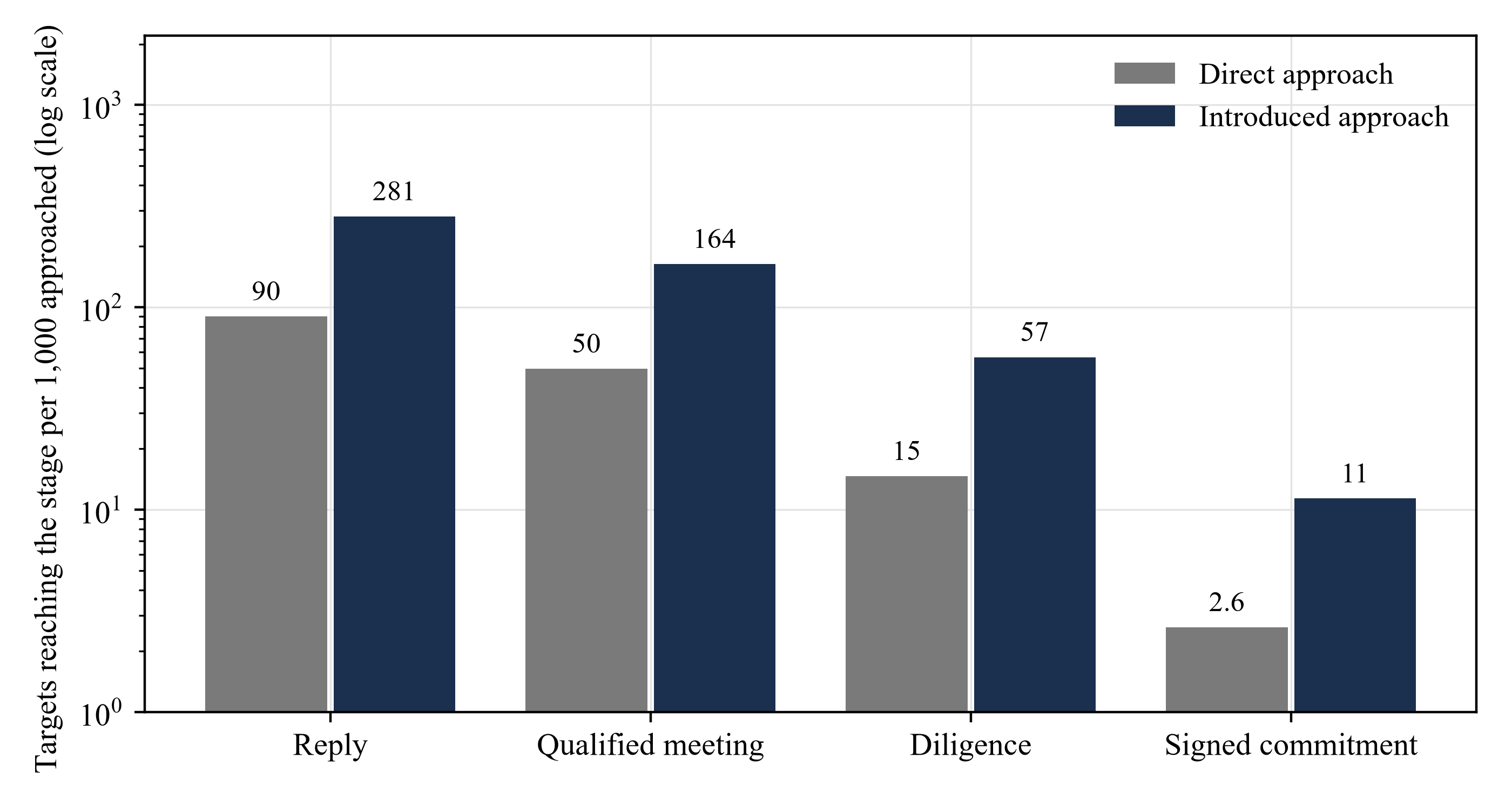
Table 5 reports the true funnel under each approach. A direct approach reaches a reply in 9.0% of targets and a signed commitment in 0.26%. An introduced approach reaches a reply in 28.1% and a signed commitment in 1.13%. The true effect is 19.12 percentage points at the reply stage, 11.39 at the qualified meeting, 4.20 at diligence and 0.87 at signature. The rate ratio rises along the ladder, from 3.12 at the reply stage to 4.33 at signature, because the log-odds effects accumulate across stages.
| Stage | Direct | Introduced | Effect (points) | Rate ratio | Effect on the introduced (points) |
|---|---|---|---|---|---|
| Reply | 9.0 | 28.1 | 19.12 | 3.12 | 24.18 |
| Qualified meeting | 5.0 | 16.4 | 11.39 | 3.30 | 15.49 |
| Diligence | 1.5 | 5.7 | 4.20 | 3.87 | 6.30 |
| Signed commitment | 0.26 | 1.13 | 0.87 | 4.33 | 1.42 |
MatchPoint analysis of the constructed population. Model output under stated inputs; not an observed result. Percentage of eligible targets approached reaching each stage; effects in percentage points.
Scroll horizontally to read the figure at full size. You can also open the full-size figure.
MatchPoint analysis of the constructed population. Model output under stated inputs; not an observed result. Log scale; rates per 1,000 approached.
The effect on the introduced group is larger than the average effect, for example 24.18 points against 19.12 at the reply stage. This is not a different mechanism. The sponsor chooses warmer, better-fitting targets, whose base rates are higher, and equal effects on the log-odds scale produce larger changes in percentage points where the base rate is higher. The first lesson for the decision is that the question of where introductions go is already part of the answer to how much they achieve. Figure 1 shows the same funnel on a logarithmic scale.
11 The raw gap between introduced and direct targets overstates the effect at every stage
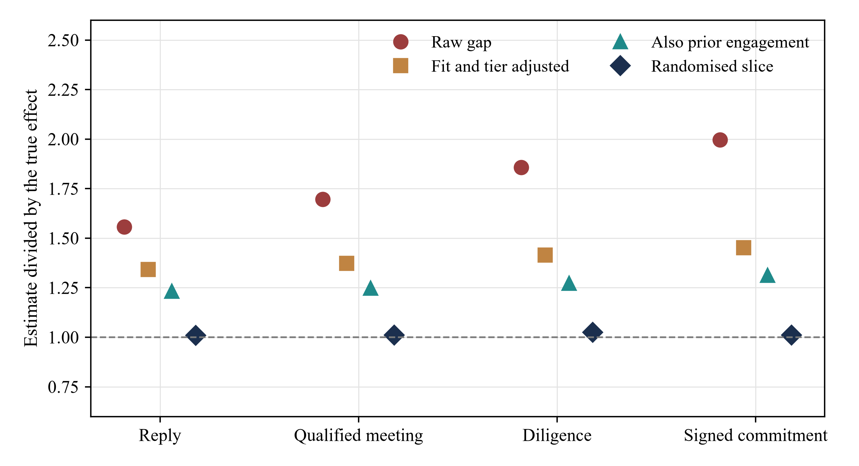
A sponsor reading its own log would compare the two groups. Table 6 shows what that comparison reports. At the reply stage the raw gap is 29.76 points against a true 19.12, a ratio of 1.56. At the qualified meeting the raw gap is 19.32 against 11.39. Applied to 100 eligible targets switched from direct to introduced approaches, the raw gap would suggest 19.3 additional qualified meetings; the constructed population-average contrast is 11.4. This average differs from the effect among targets selected for introduction. At signature the raw gap is 2.00 times the truth.
| Estimator | Reply | Qualified meeting | Diligence | Signed commitment |
|---|---|---|---|---|
| True effect (known by construction) | 19.12 | 11.39 | 4.20 | 0.87 |
| Raw gap between arms | 29.76 | 19.32 | 7.80 | 1.74 |
| Fit and tier adjusted (regression) | 25.65 | 15.65 | 5.94 | 1.27 |
| Fit and tier adjusted (weighting) | 25.68 | 15.76 | 5.97 | 1.27 |
| Also adjusted for prior engagement | 23.55 | 14.21 | 5.34 | 1.14 |
| Randomised slice | 19.29 | 11.52 | 4.31 | 0.88 |
MatchPoint analysis of the constructed population. Model output under stated inputs; not an observed result. Percentage points of eligible targets approached; estimates use large generated samples, with finite Monte Carlo variation.
Scroll horizontally to read the figure at full size. You can also open the full-size figure.
MatchPoint analysis of the constructed population. Model output under stated inputs; not an observed result. Dashed line marks a correct estimate.
The overstatement appears at every stage. Conditioning on a later stage makes matters worse. Among targets that replied, the true meeting rates are 58.1% under introduction and 55.1% under a direct approach, a gap of 3.1 points, whereas the comparison of observed introduced and direct replies reports 10.4 points. The reason is that the replying groups are different people under each approach. A comparison that starts from the stage reached, not from the target approached, answers a different question from the one the sponsor faces. Figure 2 shows each estimate as a multiple of the true effect at all four stages.
12 Adjusting for fit and tier removes 39% of the reply-stage bias, and balance on recorded variables cannot detect the rest
The standard correction adjusts for recorded fit and tier. Table 6 shows that regression standardisation gives 25.65 points at the reply stage and weighting by the estimated propensity score gives 25.68, against the true 19.12. The adjustment removes 39% of the raw bias of 10.64 points and leaves 6.53 points. At the signed stage the adjusted estimate is 1.45 times the truth. The adjustment improves the estimate and still tells a sponsor that introductions are worth 25.7 replies per 100 when the true figure is 19.1.
In equation 3a, X(i) holds recorded fit and tier, and the fitted probability p(k)(a, X(i)) comes from a logistic regression of stage attainment on the approach and X(i), then averaged over all targets with the approach set to each value. In equation 3b, e(i) is the estimated probability of introduction given X(i), clipped to lie between 0.01 and 0.99, and the two weighted means are normalised by their weights. The two estimators agree closely, 25.65 and 25.68 points, because they use the same information.
Scroll horizontally to read the figure at full size. You can also open the full-size figure.
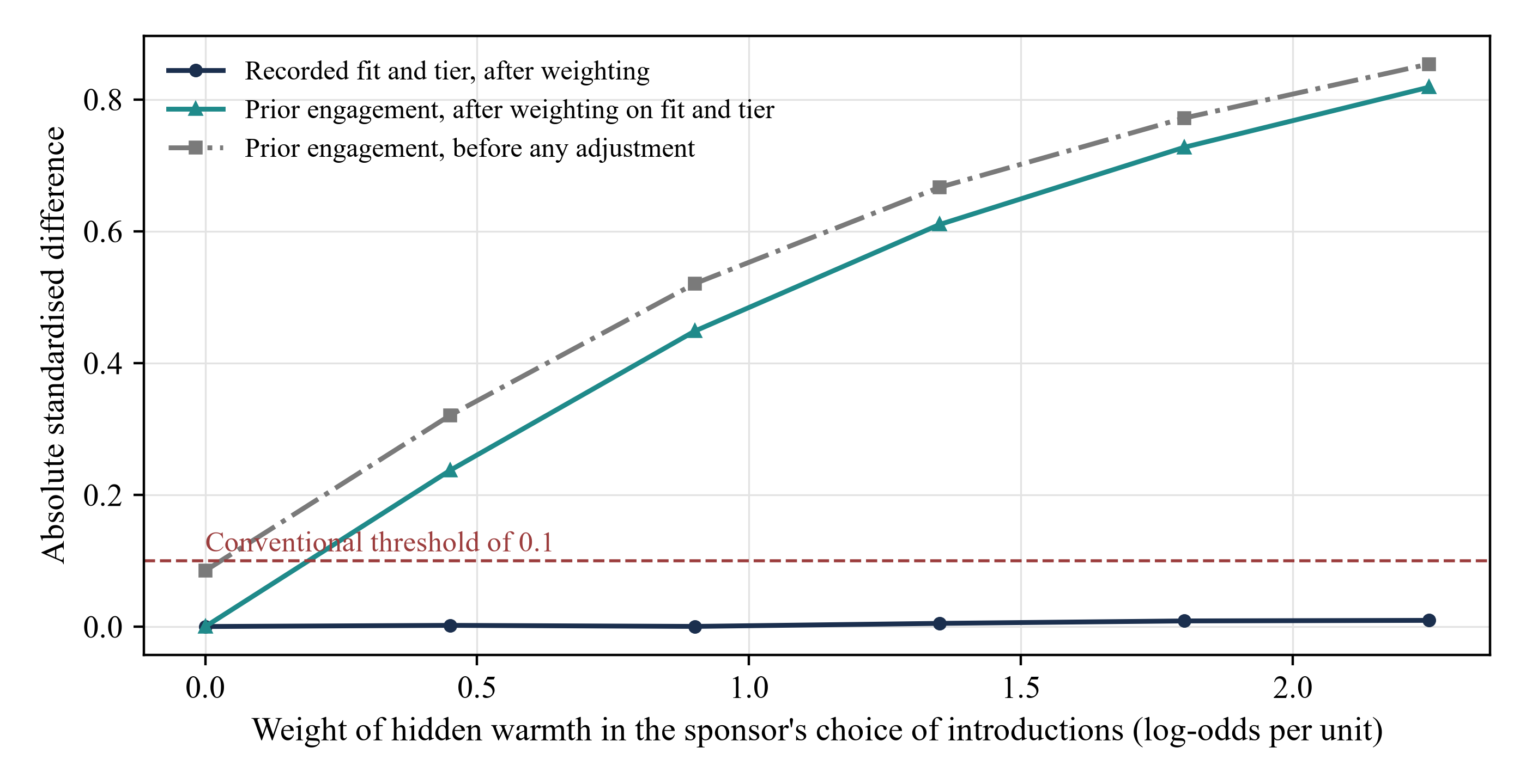
MatchPoint analysis of the constructed population. Model output under stated inputs; not an observed result. Absolute standardised differences between introduced and direct targets; the dashed line is the conventional threshold of 0.1.
Figure 3 shows why a routine balance check does not protect the sponsor. After weighting, the largest standardised difference on recorded fit and tier never exceeds 0.010 at any strength of hidden warmth, well below the 0.1 convention. [6] The prior engagement index, which responds to warmth, shows a standardised difference of 0.442 after the same weighting in the base case, against 0.513 before any adjustment. A balance table of recorded variables is clean in every case, so a clean table is not evidence that the comparison is unbiased.
13 The engagement proxy reduces bias in the base case, and the randomised benchmark is close to the constructed effect
Adding the prior engagement index to the adjustment set moves the reply estimate from 25.65 to 23.55 points and removes 58% of the raw bias. The remaining bias is 4.42 points. The proxy is a noisy measure of warmth, so it captures only part of it. The recommendation for a real study is to log any pre-contact signal of investor interest, such as opening or answering earlier correspondence, because it is the most direct available way to reduce confounding that the sponsor cannot otherwise record.
Under random assignment, warmth is balanced between arms in expectation. The population benchmark uses a separately generated sample of 400,000 targets assigned by a coin flip; it is not literally a quarter-slice of the observational population. In the repeated-campaign comparison, the observational estimators use n targets and the randomised estimator uses a separately generated sample of round(25% of n) targets from the same mechanism. The benchmark estimates 19.29 reply points, 11.52 meeting points, 4.31 diligence points and 0.88 signature points, close to the finite-population contrasts. An actual embedded slice requires random selection into the slice, adherence to assignment and compatible follow-up; discretion is surrendered within that slice.
In equation 4a, R equals one for targets in the randomised slice, and each term is the mean of the stage indicator within an arm of the slice. In equation 4b, the root mean squared error of an estimator over repeated campaigns combines its squared bias and its variance. With non-empty arms and the stated assignment mechanism, the randomised difference is unbiased in expectation for its sampled population; its realised value remains noisy. The finite code returns zero if an arm is empty. In the tested base case, adjusted estimators retain bias as sample size grows, while the randomised estimator's variance falls. Section 16 shows where the two lines cross.
14 Hidden warmth inflates adjusted estimates in the tested settings; sensitivity calculations require correctly specified confounding parameters
Scroll horizontally to read the figure at full size. You can also open the full-size figure.
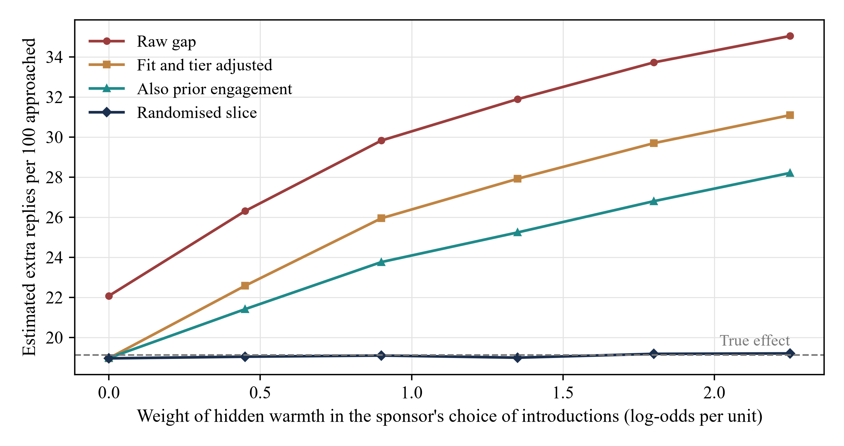
MatchPoint analysis of the constructed population. Model output under stated inputs; not an observed result. Percentage points of targets approached; the dashed line is the true effect.
Figure 4 varies the weight of hidden warmth in the sponsor's choice from none to 2.25, against the base value of 0.9. With none, the fit-adjusted estimate is 18.96 points against a true 19.12, and the raw gap is 22.07: only recorded fit and tier then confound the comparison, and adjustment repairs it. At the strongest weight tested, 2.25, the raw gap rises to 35.04, the fit-adjusted estimate to 31.09 and the proxy-adjusted estimate to 28.21. The independently simulated randomised benchmarks remain close to the generated effects, with finite Monte Carlo variation. The experiment shows how the method behaves when its premise holds, which is the case of no hidden warmth, and how far it fails as the premise weakens.
Equation 5a is the null E-value for RR greater than one. In equation 5b, the source parameters bound outcome-risk variation and confounder-prevalence variation under the stated conditioning. Their definitions involve appropriate maxima. Separately, the model's regression-standardised reply ratio is 4.26, against the generated contrast ratio 3.12, giving realised inflation 1.36. [7]
The adjusted estimate's null E-value is 7.98, and the raw estimate's is 9.58. The code also calculates within-fit-tercile and tier extrema over warmth quartiles, then population-weighted averages: 4.16 for direct-arm outcome risk and 2.66 for warmth-level prevalence. Applying equation 5b to those averages gives the descriptive number 1.90, compared with the realised ratio inflation 1.36. A median split gives 2.43, 1.79 and 1.35. These are coarsened summaries, not the theorem's uniformly bounding parameters: averaging extrema is not taking their maximum, and coarsening continuous fit and warmth leaves residual variation. Their numerical comparison does not prove a formal confounding bound or that warmth is too weak to explain the association. The known finite-population effect comes from the authored potential outcomes. The source also describes non-null E-values for shifting an estimate to a specified non-null risk ratio; a null E-value alone does not measure the realised inflation. [7]
A sponsor can use pre-contact proxy balance as a diagnostic and examine sensitivity over explicitly stated confounder associations. A standardised difference in a noisy proxy is neither a proven lower bound on hidden warmth imbalance nor the risk-ratio parameter in equation 5b. A formal sensitivity bound requires parameters and adjustment conditions appropriate to the estimand and source theorem. The constructed comparison illustrates inflation under its assumptions; it does not make adjusted estimates upper bounds in an unobserved campaign.
15 Each stress case fails with its own signature, which a sponsor can check in its own log
Table 7 reports large constructed-sample reply estimates under the base case and five stress cases. Each case uses 400,000 generated targets. The diagnostic columns measure recorded fit/tier and prior-engagement balance after weighting by recorded approach. Thus the mis-tagging case uses the same recorded approach classification as its outcome estimators. These diagnostics describe the generated records.
| Scenario | True | Raw | Fit adjusted | Also engagement | Randomised | Balance, fit and tier | Balance, engagement |
|---|---|---|---|---|---|---|---|
| Base case | 19.12 | 29.76 | 25.65 | 23.55 | 19.29 | 0.002 | 0.442 |
| No hidden warmth | 19.10 | 22.36 | 19.25 | 19.24 | 19.34 | 0.001 | 0.005 |
| Strong hidden warmth | 19.23 | 34.27 | 30.24 | 27.19 | 19.28 | 0.008 | 0.738 |
| Gains rise with warmth | 21.56 | 36.74 | 32.27 | 29.10 | 21.68 | 0.002 | 0.447 |
| Colder market | 11.57 | 18.52 | 15.73 | 14.34 | 11.49 | 0.005 | 0.440 |
| Mis-tagged introductions | 19.09 | 21.11 | 17.60 | 15.91 | 19.03 | 0.008 | 0.292 |
MatchPoint analysis of the constructed population. Model output under stated inputs; not an observed result. Percentage points of eligible targets approached; balance columns are absolute standardised differences after weighting on recorded fit and tier.
With no hidden warmth, the fit-adjusted estimate is 19.25 against 19.10, the balance on the proxy is 0.005 and the adjusted and randomised estimates agree. This is the signature of a campaign that can be read from adjustment. With strong hidden warmth the adjusted estimate is 30.24 against 19.23, the randomised estimate is unchanged at 19.28 and the proxy balance is 0.738. The signature is a large and persistent gap between the adjusted and slice estimates with a clean balance on recorded variables.
When gains rise with warmth, the true average effect is 21.56 but the effect on the introduced group is 30.99. The adjusted estimate of 32.27 sits above both, with a bias of 10.72 points against 6.53 in the base case, while the slice recovers the average effect at 21.68. The signature is an adjusted estimate that exceeds even the effect on the introduced. In a colder market, the direct reply rate falls to 4.4% and the effect to 11.57 points, while the ratio of the adjusted estimate to the truth stays near 1.36; the signature is lower rates at every stage with a similar proportional bias. When 15% of introductions are recorded as direct and 10% of direct approaches as introduced, the adjusted estimate falls to 17.60, below the truth of 19.09. The errors cancel, the answer looks right, and the cause is wrong, so the tagging audit in section 22 is a separate control.
The diagnostics can be read together. Recorded-variable balance checks only measured imbalance; proxy balance can signal a residual difference in the recorded engagement measure. The adjusted-minus-slice gap, with uncertainty and a common target population, can reveal disagreement between estimation strategies. It can also reflect sampling error, model misspecification, mis-tagging, treatment non-adherence or selection into the slice. A stage pattern may help frame further checks. None of these observations alone identifies hidden warmth or establishes that an observational comparison is unbiased.
16 In the constructed base case a 400-target campaign still has substantial estimation error
A real sponsor sees one campaign, not the population limit. The model draws 600 campaigns at each of six sizes and applies each estimator. At 400 targets the fit-adjusted reply estimate has a median of 25.59 points and a middle 80% range of 19.8 to 31.8, and 92% of campaigns overstate the true 19.12 points. The randomised slice, which here contains 100 targets, has a median of 18.42 and a range of 10.0 to 27.9. It is correct on average and unreliable in any single campaign.
| Estimator | Stage | True | Median | Middle 80% of campaigns | Estimate at or below zero | RMSE |
|---|---|---|---|---|---|---|
| Raw gap | Reply | 19.12 | 29.69 | 23.7 to 35.6 | 0% | 11.53 |
| Raw gap | Diligence | 4.20 | 7.79 | 4.5 to 11.4 | 0% | 4.60 |
| Fit and tier adjusted | Reply | 19.12 | 25.59 | 19.8 to 31.8 | 0% | 8.13 |
| Fit and tier adjusted | Diligence | 4.20 | 5.89 | 2.9 to 9.5 | 0% | 3.13 |
| Also engagement | Reply | 19.12 | 23.50 | 17.6 to 29.6 | 0% | 6.45 |
| Also engagement | Diligence | 4.20 | 5.33 | 2.4 to 8.7 | 0% | 2.74 |
| Randomised slice (100 targets) | Reply | 19.12 | 18.42 | 10.0 to 27.9 | 0% | 7.15 |
| Randomised slice (100 targets) | Diligence | 4.20 | 4.00 | 0.0 to 8.7 | 14% | 3.66 |
MatchPoint analysis of the constructed population. Model output under stated inputs; not an observed result. Percentage points; the middle 80% range is the 10th to 90th percentile over 600 campaigns; RMSE is the root mean squared error against the true effect.
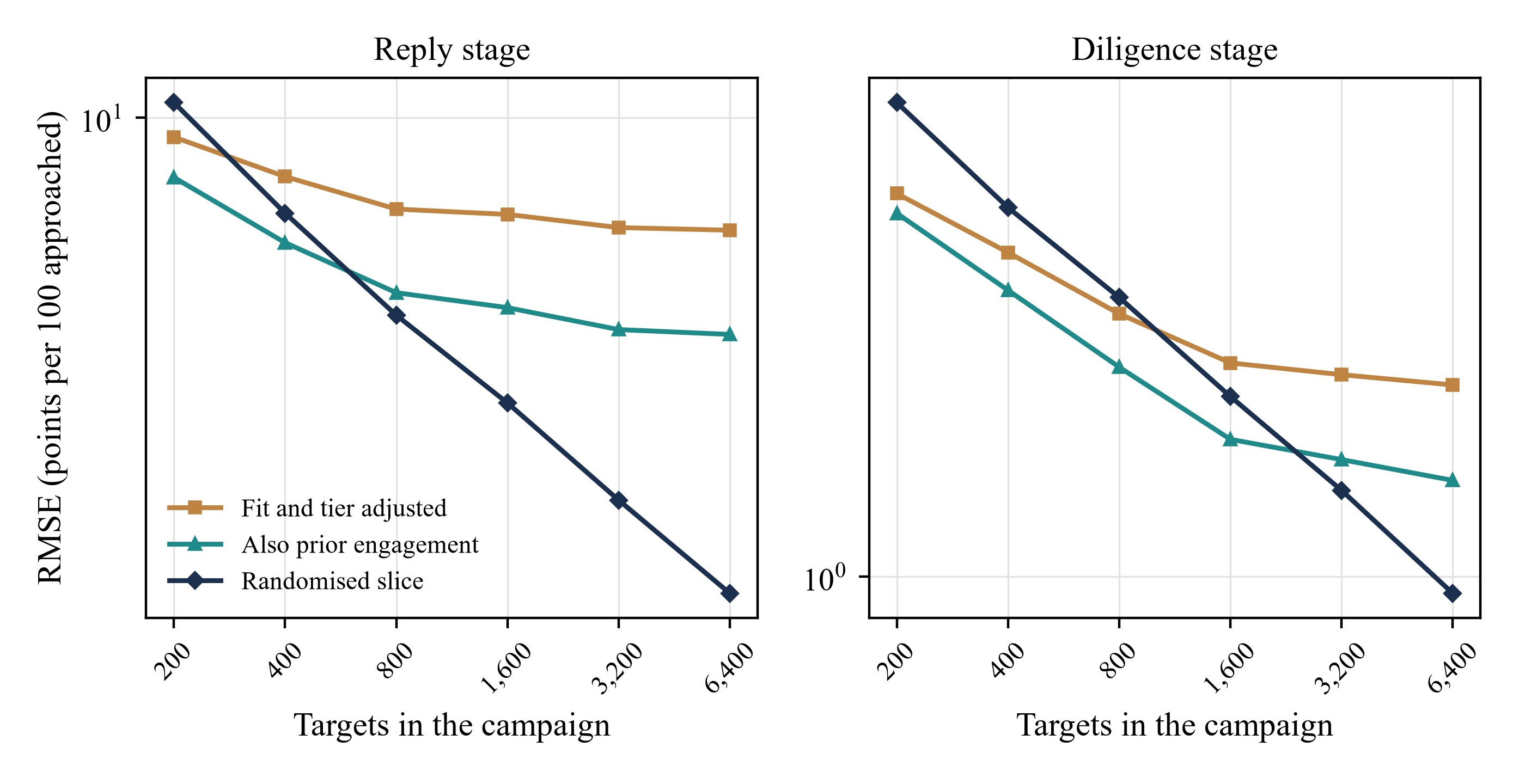
Scroll horizontally to read the figure at full size. You can also open the full-size figure.
MatchPoint analysis of the constructed population. Model output under stated inputs; not an observed result. Root mean squared error in percentage points per 100 approached; both axes logarithmic; randomised slice is 25% of the campaign.
Table 8 and Figure 5 show the trade between bias and noise. At 400 targets the fit-adjusted error at the reply stage is 8.13 points against 7.15 for the slice, so the slice is already the better estimate at 400 targets. At 6,400 targets the fit-adjusted error has barely fallen, to 6.74, while the slice error has fallen to 1.88. With the proxy added, the slice overtakes at 800 targets. At the diligence stage the crossing occurs at 1,600 targets. These are the first crossing points on the six tested campaign sizes under this construction, not continuous threshold estimates or a general rule for a sponsor. A real choice depends on its assignment mechanism, effect sizes, precision and available randomised sample.
17 Under the authored rates, later endpoints require larger randomised samples
In equation 6a, p(1) and p(0) are the true stage rates under introduction and direct approach, z are standard normal quantiles for a two-sided test at the 5% level and power of 80%, and n(arm) is the number of targets needed in each arm of the slice. In equation 6b, s is the share of the campaign that is randomised, set at 25%, and N(campaign) is the number of targets the whole campaign must approach. The formula is an independent-target normal approximation, and the formula-sized simulation checks only the reply stage. Coin-flip allocation gives expected rather than fixed arm counts. The simulated Wald rejection rule uses both tails, treats zero estimated standard error as non-rejection and can be poorly calibrated for rare endpoints; these sample sizes require endpoint-specific validation before use.
| Endpoint | Direct (%) | Introduced (%) | Targets per arm for 80% power | Campaign size at the stated slice | Campaigns of 400 | Simulated power, n = 400 | Simulated power, n = 6,400 |
|---|---|---|---|---|---|---|---|
| Reply | 9.0 | 28.1 | 62 | 496 | 1.2 | 73% | 100% |
| Qualified meeting | 5.0 | 16.4 | 112 | 896 | 2.2 | 46% | 100% |
| Diligence | 1.5 | 5.7 | 302 | 2,416 | 6.0 | 16% | 100% |
| Signed commitment | 0.26 | 1.13 | 1,428 | 11,424 | 28.6 | 0% | 55% |
MatchPoint analysis of the constructed population; not an observed result. Approximate independent-target normal-formula sizes at a 5% two-sided level and 80% target power; simulated Wald rejection rates use the stated campaign sizes and can be poorly calibrated for rare endpoints.
The reply stage needs 62 targets per arm, which a campaign of 496 approaches provides at the stated slice. The qualified meeting needs 112 per arm and 896 approaches, and diligence needs 302 per arm and 2,416 approaches, about 6 campaigns of 400. A signed commitment needs 1,428 per arm and 11,424 approaches, about 29 campaigns of 400. At 400 targets the simulated power is 73% at the reply stage, 46% at the qualified meeting and 16% at diligence. Under these authored rates, early endpoints need fewer targets than later endpoints. Actual inference requires the interval and achieved sample size. Pooling mandates also requires comparable definitions, attention to mandate heterogeneity and correlated targets, and an appropriate analysis; the independent-target formula does not account for these features.
18 Where introductions are scarce, the constructed effect is largest for well-fitting targets outside the hardest tier
A sponsor with a fixed number of introductions needs to know where each is worth most. Table 10 reports the true effect of an introduction by fit tercile and tier. In the constructed world the effect at the reply stage ranges from 10.0 extra replies per 100 for low-fit targets in the first tier to 26.7 for high-fit targets in other tiers. The effect at the qualified meeting ranges from 7.0 to 17.9 extra meetings per 100 introductions in other tiers.
| Fit tercile | Other tiers: extra replies | Other tiers: extra meetings | Tier 1: extra replies | Tier 1: extra meetings |
|---|---|---|---|---|
| Low fit | 14.5 | 7.0 | 10.0 | 4.9 |
| Middle fit | 20.7 | 12.0 | 15.1 | 8.6 |
| High fit | 26.7 | 17.9 | 21.6 | 14.4 |
MatchPoint analysis of the constructed population. Model output under stated inputs; not an observed result. True effects in percentage points, by fit tercile and tier; cells reconcile to the population effect. A template for a slice result: the pattern follows from equal log-odds effects and is not a finding.
The pattern is a consequence of the construction. Effects are equal on the log-odds scale, and the base rates are low, so the percentage-point effect is larger where the base rate is higher: at better-fitting targets and outside the first tier. A real matrix could look different, for example if introductions matter most for hard-to-reach investors. The table is therefore a template for a result that the randomised slice can produce, not a finding. A sponsor needs the slice to be large enough to estimate cell effects, which is more than the overall effect requires.
19 Reproduction, controls and what the experiment cannot show
The numerical model uses the fixed seed 1377 and asserts 47 controls, summarised in Table 11. These check the selection identity, stage nesting, stated calibration tolerances, finite randomised benchmark errors, E-value arithmetic, reconciliation of matrix cells and a reply-stage normal-formula power check. The sensitivity-summary controls check arithmetic and a realised comparison in this construction; they do not certify a formal confounding bound.
| Control | Expected result |
|---|---|
| Fixed seed | Seed 1377; repeating a campaign with the same key reproduces every estimate exactly |
| Generated probabilities | Strictly between zero and one at every stage in every scenario |
| Stage nesting | Signed within diligence within meeting within reply, for both potential outcomes, for every target |
| Calibration | Direct-arm stage rates equal the stated inputs within four standard errors |
| Introduced share | 30% within 0.003 in the population |
| Selection identity | Raw gap equals the effect on the introduced plus the selection term, to 1e-12, at all four stages |
| No hidden warmth | Fit-adjusted estimates within 0.004 of the true effect at every stage |
| Randomised slice | Within 0.004 of constructed truth in the population benchmarks; simulated reply-stage mean error below 0.005 at n = 6,400 |
| Balance rule | Weighted standardised differences on fit and tier below 0.1 in every scenario |
| E-value arithmetic | E-value of 1 is 1; of 2 is 2 + sqrt(2); unchanged by inversion; descriptive summary-factor arithmetic checked |
| Scoring matrix | Cell sizes sum to the population; weighted cell effects reconcile to the population effect |
| Power formula | Formula-sized slice delivers simulated power within 0.08 of 0.80 |
| Checks asserted in model.py | 47 identities and boundary tests passed |
MatchPoint analysis of the constructed population. Model output under stated inputs; not an observed result.
The experiment cannot show whether introductions work in any real market. The potential outcomes are generated from the same variables that the methods use, so the experiment shows how the methods behave when the generating assumptions hold, not that those assumptions hold. The true effect, the strength of hidden warmth, the loading of the proxy and the funnel rates are authored. A reader should take from it the direction and relative size of the biases and the sample sizes involved, and should not read the percentages as estimates of what introductions achieve in Gulf or global private markets.
Two limits of the controls deserve statement. A passed identity shows that the code implements the stated equations, not that the equations describe investor behaviour. The replications use 600 campaigns per size, so the reported ranges carry Monte Carlo error that is small relative to the gaps discussed but not negligible at the smaller sample sizes.
20 A consented study needs a logged slice, tagged introductions, stage timestamps and a stated analysis plan
A real study would run inside a sponsor's live campaigns, with the permission of the sponsor, the introducers and, where required, the investors whose data are recorded. The unit is the pair of one target and one mandate. The study is not a survey of investors and does not require them to alter their behaviour, but the sponsor should confirm the lawful basis for recording engagement and the basis on which it contacts each target. Zhang reports that his consented experiment, in which investors were told the research purpose, probably understates bias because of a consent form effect, and that he did not recruit European Union investors for his pitch-email experiment because of the General Data Protection Regulation. [5]
| Element | Specification | Reason |
|---|---|---|
| Unit | One target for one mandate | Stage clocks differ by mandate |
| Eligibility | A named introducer path exists before assignment | Keeps the comparison to targets that can be introduced |
| Assignment | Logged coin flip for a share of eligible targets; remainder at discretion | Removes warmth from the slice; keeps sponsor judgement elsewhere |
| Timestamps | First contact and each stage, from system records | Same clock for every arm |
| Tags | Approach type and introducer tie recorded at source | Supports approach-type verification and a mis-tagging audit |
| Pre-contact signals | Prior engagement and recorded fit, fixed before assignment | Enables diagnostics and proxy adjustment |
| Consent and data | Lawful basis recorded per target; objection honoured | Consent standards in the sources reviewed |
| Sample size and analysis | Slice sized by equation 6; effects with intervals; adjusted estimate only as a secondary | Supports interpretation using estimates and intervals |
Proposed specification. Entries describe design choices to be fixed in advance; they are not findings.
Table 12 lists the design elements. The analysis plan is registered before the first approach. It states the four stage endpoints, the clocks, the primary estimator (the slice difference), the secondary estimator (adjustment with the proxy), the tests for mis-tagging, and the rule for pooling campaigns. Zhang's study was registered in the AEA RCT Registry, which is the practice a sponsor can follow in spirit by dating its plan. [5] A study that finds no effect at the later stages should report the interval and the sample size, since an interval that includes both zero and a material effect is a reason to pool, not a reason to conclude.
21 Report the slice effect, the adjusted effect and the gap between them to the board or investment committee
The committee report should present the slice effect with its interval, the adjusted effect, and their difference with uncertainty, using a common target population and endpoint. In the base case the adjusted reply estimate is 1.34 times the known effect, while the randomised benchmark is close to it. In a real study the gap can reflect sampling variation, model specification, assignment adherence, measurement or slice selection as well as unmeasured confounding. Agreement on replies does not validate adjustment for later endpoints; those require their own identification and precision assessment.
| Item | Content | Decision supported |
|---|---|---|
| Slice effect | Difference with interval at each stage reached | Whether introductions change early progress |
| Adjusted effect | Estimate with fit, tier and engagement; method stated | An endpoint-specific association unless its identification assumptions are supported |
| Gap | Adjusted minus slice, with the diagnostic on engagement | Potential disagreement between strategies, assessed with uncertainty and comparable populations |
| Stage pattern | Effects by stage and by cell | Where introductions open doors and where they close mandates |
| Tag audit | Share of introductions with a verified tie record | Whether the arms are defined correctly |
| Capacity | Introductions available and used, by tier | Whether more introductions can be obtained |
Proposed report contents. Entries describe information to present; they are not findings.
Table 13 lists the contents. The report should say what the committee should not conclude. A positive effect at the reply stage is not evidence of a positive effect on signed commitments, which take far more targets to measure. A positive average effect is not evidence that any particular introduction will work. A report that omits the interval invites the reading that the point estimate is proof. Each of these limits is visible in the constructed experiment, in which the sample sizes of Table 9 show how little a single raise can establish.
22 Use data and AI to maintain tie records and diagnostics, and keep human control of who is approached
The inputs to this test are records: who knows whom, when an approach was made, what the investor did and when. Software can maintain those records by extracting dates and senders from correspondence, tagging the approach type and flagging gaps. These are proposals; this paper reports no tool, accuracy or benefit from AI. A tagging system should be tested against a hand-checked sample, since the mis-tagging stress case shows that errors of 10% to 15% can move an adjusted estimate below the truth and make it look correct.
A warmth score derived from correspondence could be evaluated as a pre-contact proxy. Its feature window and model version should be fixed before assignment. Post-approach messages must not enter a baseline adjustment variable. If the score also informs discretionary introductions, its role belongs in the recorded assignment mechanism. The proposed randomised component remains separately assigned and audited. The paper measures no AI accuracy or commercial benefit.
Human decision rights remain explicit. The sponsor decides which targets are eligible and who approaches them. The introducer decides whether to make an introduction and with what wording. Compliance confirms the legal basis for each approach. A model may prepare the records and the diagnostics, and none of these decisions should be delegated to it.
The proposed tag audit compares the sponsor's record with the introducer's retained message on a pre-specified sample and records agreement and error direction. In the constructed stress case, 15% of introduced approaches and 10% of direct approaches are misclassified, materially changing the adjusted estimate. A real audit needs its own sample and uncertainty assessment. Its cost is not estimated here.
23 Apply a decision rule in a live raise: slice early, pool later, and spend introductions where the slice says they matter
A proposed operating sequence starts with eligible targets, recorded baseline characteristics, lawful contact and processing bases, and defined outcomes. Random selection into the experimental component and random assignment within it should be logged before approaches. Discretionary approaches remain separately tagged. Follow-up uses comparable elapsed windows, with deviations, repeated targets and missing records retained for analysis. Figure 6 outlines the sequence. Validity depends on adherence, outcome measurement and the assumptions stated above.
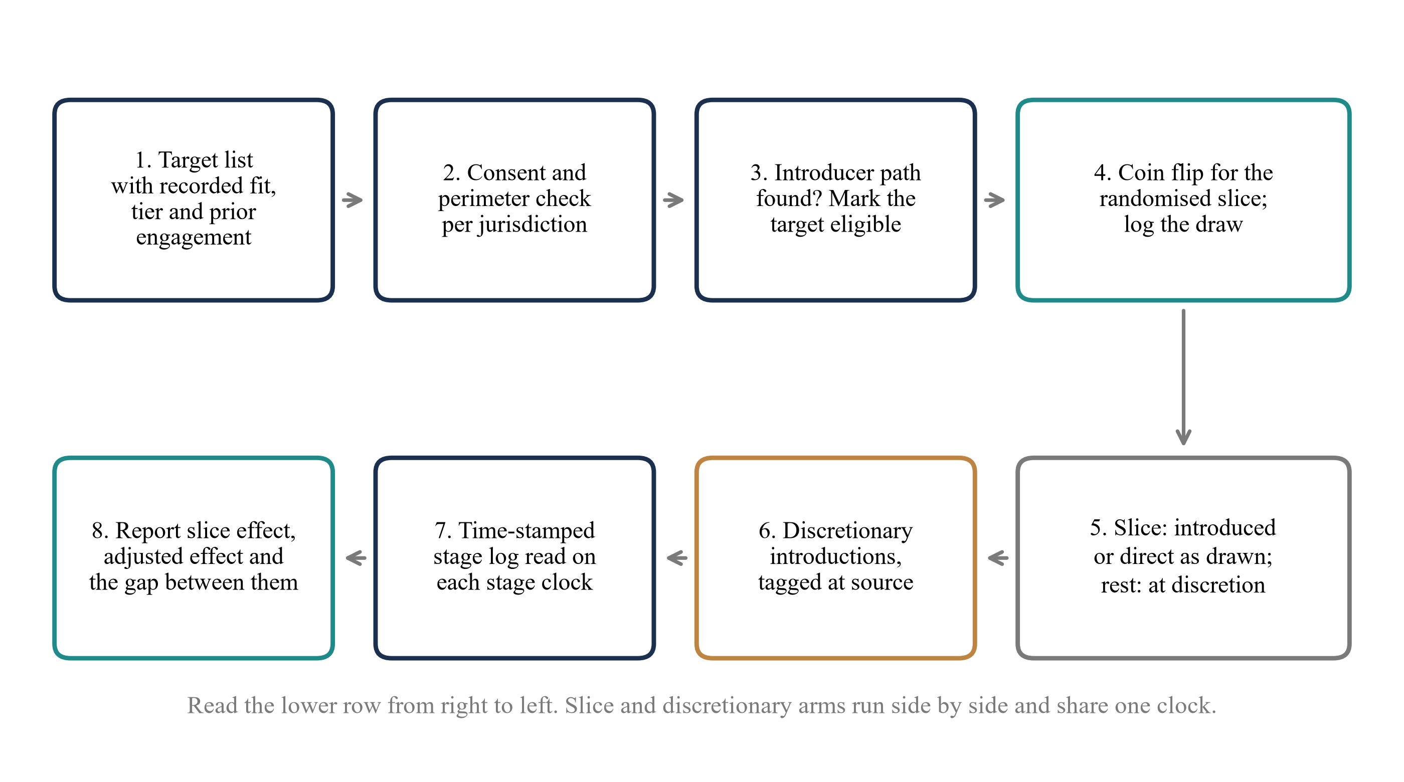
Scroll horizontally to read the figure at full size. You can also open the full-size figure.
MatchPoint analysis. Proposed sequence for a study inside a live campaign; not an observed result.
| Condition | Action | Evidence that triggers it |
|---|---|---|
| Under the authored rates and approximately 500 eligible independent targets | Assess endpoint-specific power and uncertainty; later-stage estimates may remain imprecise | Sample size of equation 6 |
| Adjusted and slice estimates agree within the interval | Assess uncertainty and identification at each endpoint; do not validate later-stage adjustment from early agreement alone | Endpoint-specific estimates, intervals, diagnostic balance and justified identification assumptions |
| Adjusted estimate exceeds the slice estimate by a wide margin | Do not plan on adjusted estimates; enlarge the slice | Gap and engagement balance |
| Introductions are scarce | Place them where the slice shows the largest effect per introduction | Cell estimates, pooled across mandates |
| Introducer is rewarded | Review the applicable activity, promotion and compensation rules before an approach; verify any exemption in full | Sources on introducer rewards |
| Stage results pooled across mandates | Use common endpoints and assess mandate heterogeneity, repeated targets and clustering in the pooled analysis | Common ladder and clocks |
Proposed rule. Thresholds are for the sponsor to set in advance; none is a finding.
Table 14 sets out the rule. The rule has a cost. A slice of 25% means that a quarter of the eligible targets are assigned by a coin flip and not by the sponsor's judgement. The experiment shows the bias that the slice avoids, which the adjusted estimators retain in the tested base-case campaign-size grid, but it does not price the cost. Whether a particular sponsor should pay it depends on how many introductions it holds and how many mandates it can pool, which are facts the sponsor knows and this paper does not.
24 Limitations and the next decision: replace the authored effects with a logged slice
The experiment is constructed. Its funnel rates, effect sizes, strength of hidden warmth and proxy loading are authored, and its conclusions about the direction of bias follow from stating that introducers act on warmth the record cannot see. The population contains one hidden variable and one proxy; a real campaign has many. Effects are equal on the log-odds scale, which fixes the pattern in the scoring matrix. Targets do not influence one another, though investors in one syndicate or one network may. No source reviewed measures the prevalence or effect of introductions among Gulf investors.
The sources have their own limits. The survey of venture capital investors is a working paper and describes deal origination, not outcomes after the same approach. The referral experiments concern labour, and the investor pitch experiments stop at the first reply and concern cold email. The Gulf data protection texts other than the ADGM guidance and a government portal summary were not read, and the regulators' rulebooks on marketing were not reviewed beyond a DFSA public alert. Each of these is a limit on what the framework may be used for.
The decision that follows is specific. A sponsor with introductions to spend should begin the next campaign with a logged slice at the early stages, with tagged introductions and a pre-contact engagement record throughout. Under the authored independent-target assumptions, the approximate design sizes are 496 total targets for replies and 896 for qualified meetings, with larger samples for later endpoints. Real studies require endpoint-specific uncertainty, follow-up and pooling assessments. Raw and adjusted gaps can lie above or below the causal effect; the mis-tagging scenario itself places the adjusted reply estimate below it. Treat these gaps as associations unless identification assumptions are justified. The descriptive coarsened sensitivity summaries in section 14 do not provide certified upper bounds.
The audience should also note what the paper leaves out. It does not rank investors, which is a separate question from whether an introduction changes progress, and it does not price an introduction. It treats an introduction as one bundle and does not separate the information an endorsement carries from the access it provides. It does not model the introducer's incentives, which the conditions on rewards in section 7 suggest may matter. Each is a candidate for the next study once a logged slice exists.
References
- Gompers, P., Gornall, W., Kaplan, S. N. and Strebulaev, I. A. How Do Venture Capitalists Make Decisions? NBER Working Paper 22587, September 2016, section 3.1 and Tables 5 and 6. Working paper; later published in a journal, published version not reviewed. https://www.nber.org/system/files/working_papers/w22587/w22587.pdf
- Shane, S. and Cable, D. Network Ties, Reputation, and the Financing of New Ventures. Management Science 48(3), March 2002, pp. 364-381. Bibliographic record and abstract only. https://ideas.repec.org/a/inm/ormnsc/v48y2002i3p364-381.html
- Pallais, A. and Sands, E. G. Why the Referential Treatment? Evidence from Field Experiments on Referrals. NBER Working Paper 21357, July 2015; published in the Journal of Political Economy 124(6), 2016. Working paper text read; published version not reviewed. https://www.nber.org/system/files/working_papers/w21357/w21357.pdf
- Gornall, W. and Strebulaev, I. A. Gender, Race, and Entrepreneurship: A Randomized Field Experiment on Venture Capitalists and Angels. Management Science 71(6), June 2025, pp. 5308-5327. Published abstract read; full text read in the August 2019 working-paper version (AEA 2020 conference copy). https://ideas.repec.org/a/inm/ormnsc/v71y2025i6p5308-5327.html
- Zhang, Y. Discrimination in the Venture Capital Industry: Evidence from Two Randomized Controlled Trials. arXiv 2010.16084, version dated 14 March 2022. Working paper; read in part (introduction, design notes, footnotes). https://arxiv.org/pdf/2010.16084v1
- Austin, P. C. An Introduction to Propensity Score Methods for Reducing the Effects of Confounding in Observational Studies. Multivariate Behavioral Research 46(3), 2011, pp. 399-424. Open-access text on PubMed Central. https://pmc.ncbi.nlm.nih.gov/articles/PMC3144483/
- VanderWeele, T. J. and Ding, P. Sensitivity Analysis in Observational Research: Introducing the E-Value. Annals of Internal Medicine 167(4), 2017, pp. 268-274. Author manuscript, including appendix on non-null E-values. https://dash.harvard.edu/server/api/core/bitstreams/7312037e-0f45-6bd4-e053-0100007fdf3b/content
- U.S. Securities and Exchange Commission, Division of Corporation Finance. Securities Act Rules, Corporation Finance Interpretations, Questions 256.26 to 256.32; individual interpretation dates 6 August 2015 and 12 March 2025. Staff interpretations; accessed 16 November 2026. https://www.sec.gov/rules-regulations/staff-guidance/corporation-finance-interpretations/securities-act-rules
- United Kingdom. The Financial Services and Markets Act 2000 (Financial Promotion) Order 2005, SI 2005/1529, Article 15. Official revised XML, including paragraph 1A and paragraph 2; accessed 16 November 2026. https://www.legislation.gov.uk/uksi/2005/1529/article/15/data.xml
- European Union. Regulation (EU) 2016/679 (General Data Protection Regulation), Articles 4, 7 and 21. Official Journal L 119, 4 May 2016. https://eur-lex.europa.eu/legal-content/EN/TXT/HTML/?uri=CELEX:32016R0679
- Abu Dhabi Global Market, Office of Data Protection. Lawful Bases for Processing Personal Data and Special Categories of Personal Data. Guidance brochure, May 2025. Regulator guidance, not the text of the Regulations. https://assets.adgm.com/download/assets/ADGM+Lawfulness+of+Processing+Brochure.pdf/643e101658a711ef9ce5e27828504259
- United Arab Emirates Government Portal. Data protection laws: summary of Federal Decree Law No. 45 of 2021. Official summary accessed 16 November 2026; the full statute was not reviewed. https://u.ae/en/about-the-uae/digital-uae/data/data-protection-laws
- Mubadala. Contact us, section on spam and potentially improper conduct. Company page accessed 16 November 2026; the cited passage is a fraud warning. https://www.mubadala.com/en/contact-us
- Dubai Financial Services Authority. Unauthorised Business in the DIFC. Alert, 1 June 2023, describing Articles 41 and 41A of the Regulatory Law 2004. Regulator alert, not the Rulebook text. https://www.dfsa.ae/alerts/unauthorised-business-difc
About the Author
Chennakeshav (CK) is a corporate finance and investment banking executive with 25+ years of global experience in deal origination, structuring and execution across M&A, growth capital and corporate strategy. He has led value-creation mandates for founders, corporates and funds — bridging the boardroom view to hands-on execution and close.
His career spans Morgan Stanley, HSBC, Lloyds Banking Group, EWEC, ADQ portfolio companies and Emirates Growth Fund, across TMT, real estate, fintech, deeptech, cleantech, infrastructure and energy. He has partnered with C-suite leaders, private equity and venture funds, sovereign wealth funds and family offices to finance complex fund raises and scale-up ventures, and has led M&A due diligence, post-merger integration and business-transformation initiatives to create value.
At Matchpoint Partners he is Managing Partner, leading the firm's corporate finance, M&A and capital-raising practice. He holds an MBA from London Business School, an engineering degree from VTU and a Master of Laws (LLM, in progress) from UCL London.
An active start-up mentor, CK mentors at Techstars, DIFC FinTech Hive, Startup Grind, Founder Institute and IN5, serves as Entrepreneur Mentor in Residence (EMiR) at London Business School, and judges the Entrepreneurship World Cup.
https://www.linkedin.com/in/ckadya/
https://www.matchpoint-partners.com/team/ck-adya.html
Disclaimer
This paper is part of a continuing series on the structure of private and alternative markets. The views expressed are the author's own. The paper is for information only, describes market structure in general terms, and does not constitute investment, legal, tax or regulatory advice or a recommendation in respect of any security, vehicle or counterparty.
