

1 Rank investors by whether they can commit in the window, then by fit
A raise has a closing date, a ticket size and a list of investors that is longer than the team can approach in one wave. The decision is the order of approach. Mandate fit answers whether an investor would buy this kind of asset. It does not answer whether the investor has room to buy it now, or whether its committee can approve before the window closes. This paper studies those two further questions, capacity and timing, and asks which observable variables are most useful for ranking a constrained investor universe once fit has been settled.
We hold no observed outreach dataset. The paper therefore does three things. It reads primary institutional documents to establish which capacity and timing variables an investor publishes, with what lag and with what ambiguity. It builds an authored experiment on a constructed universe of 1,600 plus 2,000 investors per replication, repeated 100 times, in which capacity, pacing and committee calendars are generated from stated inputs and observed only through lagged and incomplete records. It then specifies the consented study that would replace the constructed universe with evidence.
The experiment reports model results under stated inputs. It is not a market observation. Where a sentence below says that a ranking rule performs better, it means that it performs better in the constructed universe, whose generating assumptions are listed in full. The first third of the paper builds the variables from sources. The middle measures what each variable adds. The final third turns the result into a reporting pack, a data and governance design, and a decision rule for a live transaction.
2 Define the outcome and the clock before choosing any variable
The target outcome is an executed, legally binding commitment for at least 25 million US dollars within twelve months of launch. The instrument must create the investment or financing obligation under the transaction documents; a side letter, meeting or non-binding indication alone is insufficient. Qualified first meetings and diligence starts are recorded separately. A final decline is treated as a competing event only under a pre-specified closure rule. A contact that pauses, asks for different terms or requests a later approach remains in its appropriate open state. Every approached investor remains in the campaign denominator. [14]
The clock matters as much as the outcome. A commitment signed in month thirteen counts as a failure of the window even though the investor was willing and able. The window is measured from the launch date, and the approach month is a recorded decision, not a nuisance variable, because Section 15 shows that the same investor has different odds of committing depending on when it is approached. Table 1 states the three events, the day each is counted and the rule for investors that never respond. Recording the approach month also allows a later analysis of whether late approaches fail because the window closes or because the investor's budget has already been used.
| Event | Counted when | Counting rule | Competing outcome |
|---|---|---|---|
| Qualified meeting | First substantive meeting held | Date of the meeting, once per investor | Final decline that closes the recorded investor and raise episode |
| Diligence started | Data request or process opened by the investor | Date of the first formal request | Final decline after the meeting under the pre-specified closure rule |
| Binding commitment | Executed instrument creating an obligation for at least the ticket | Execution date at or before the fixed closing deadline | Final decline before commitment; approvals after the deadline are outside-window follow-up |
| No response | No recorded response by the last observation date | Retained in the approached denominator and administratively right-censored at the pre-specified horizon | Silence alone is not a competing decline |
Authored definitions for the constructed experiment and the proposed study. A qualified meeting requires the named decision-maker or an investment team member with authority to progress; a call with a gatekeeper does not count. The simulation generates funnel indicators and committee eligibility. Actual event timestamps and censoring belong to the separately proposed prospective study.
Two features of this definition drive the design. First, the commitment is conditional on a chain of events, so a variable can be useful for one link and useless for the next. Section 14 measures that directly: the same investors are followed from first meeting to signature under each ranking rule. Second, the competing-risk structure means that a naive success rate among responders overstates the rate among everyone approached, and a cumulative incidence calculation is the appropriate summary of time to commitment. [14]
3 Published allocation targets and ranges give the direction of capacity, not its size
Policy exposure and current decision capacity are distinct records. The marked-up November 2022 CalPERS attachment provides a historical example of allocation ranges and temporary deviations; its private-equity target is not a current input. The June 2026 consultant review reports a 20.0% private-equity allocation against a 17% long-term target and states that the portfolio remains within its five-percentage-point range. The same review records USD 15.4 billion of net new commitments over the first three fiscal quarters. A position above the central target can coexist with continued commitments. An analyst must establish the applicable range and denominator rather than treat the target itself as an automatic stop. [1, 19]
These documents establish two things for ranking. A range is a durable signal of appetite, and a change in the range is a dated event that a team can observe. They also establish a limit. A range is not a weight: the review pages we opened state ranges and do not state the weight actually held. A policy attachment is also a snapshot. The consultant's June 2025 memorandum to the same CalPERS committee refers to a long-term private equity target of 17 per cent, while the November 2022 attachment lists 13 per cent in its strategic allocation table. The memorandum records that the board approved the 17 per cent long-term target in March 2024, and the attachment is a marked-up draft, so we draw only the lesson that targets are revised and must be dated before use. [1, 3]
Allocation headroom is a candidate input where both policy limits and dated exposure are disclosed. Missing records require an explicit assumption. In the fitted score, missing numerical features receive the training mean after standardisation. The structural score uses a type-specific target exposure default, a fixed unfunded ratio of 0.25 of that exposure and a fixed distribution yield of 0.15. These are different imputations and are reported separately. Public policy documents support the choice of categories. They provide no universal weight, tolerance band or threshold for an investor’s willingness to commit.
4 A published commitment budget is the most direct pacing signal, and few investors disclose one
Pacing is the rate at which an investor commits to a strategy. The CalPERS private equity programme review dated 16 June 2025 states that commitments have been consistent with a target of 15.5 billion US dollars a year, plus or minus 15 per cent, for the last four fiscal years, and that maintaining a minimum level of commitments is important to avoid another lost decade. The consultant's memorandum reports 19.6 billion dollars of new commitments in the twelve months to 31 March 2025, including 12.0 billion dollars of co-investments alongside 50 new fund commitments, and a pace above 15 billion dollars a year over the last three years against 3 to 5 billion dollars a year in 2016 to 2018. [2, 3]
The annual commitment target supplies a flow measure alongside the portfolio stock. The 2025 staff review reported a USD 15.5 billion annual target and USD 92.1 billion of private equity net asset value, with different measurement dates. Their ratio is approximately 16.8%. The experiment retains a common authored pace parameter of 17% of target stock for all four simulated investor types. This transfer across types is a modelling assumption. It provides no estimate of the actual budgets of sovereign investors, pensions, endowments or family offices. [2]
Gulf sovereign disclosures are less granular. Mubadala reported capital deployed of AED 143 billion, up 20 per cent, and proceeds of AED 138 billion, up 27 per cent, for 2025, in a release of 9 April 2026. Proceeds equal about 97 per cent of deployment on those figures, which shows that, in that year, realisations were of the same order as deployment at that investor. The release does not split deployment by asset class or fund commitments, so it supports a pacing prior and not an investor-level budget. [6]
The June 2026 review provides a useful update. Staff retained the USD 15.5 billion annual target, with a 15% band, and reported USD 119.3 billion of private equity NAV at 31 March 2026. Dividing the same target by the newer NAV gives approximately 13.0%. A parameter inferred mechanically from that ratio would change even though the disclosed annual target had remained the same. A working record therefore needs the numerator’s period, the denominator’s valuation date and the precise portfolio perimeter. A disclosure refresh should preserve all three. [18]
5 Unfunded commitments and distributions determine when headroom reopens
A commitment is not an investment. Capital is called over several years, and the position builds as calls arrive and falls as distributions are paid. A recent optimisation paper on illiquid alternatives states the structure plainly: the investor controls only commitments, the effect on positions is delayed by typically a few years, and capital calls must be met from liquid assets. It cites the discrete-time model of Takahashi and Alexander, in which calls are a time-varying fraction of uncalled commitments. The paper is an unreviewed preprint, and we use it for the structure of the problem, not for any parameter. [12]
Two observable ratios follow. The unfunded commitment ratio, uncalled commitments over net asset value, measures capital already promised. The distribution yield measures recycling. The Institutional Limited Partners Association principles ask for estimates of quarterly projections of capital calls and distributions from the manager, and for a cap or monitoring threshold on recycling so that investors can project cash requirements. The CalPERS review lists reducing the ratio of unfunded commitments to net asset value among its aims and records that distributions have been well below historical levels. [2, 8]
Robinson and Sensoy study 837 buyout and venture funds from 1984 to 2010. Their working-paper results associate capital calls and distributions with public equity valuations, with a greater response in distributions. In their buyout net-cash-flow decomposition, age and calendar-quarter effects account for 7.9% of variation, including 7.2 percentage points from age. The remaining residual variation does not establish that other information is uninformative or that future flows are intrinsically unpredictable. The result supports caution about simple forecasting rules within that study’s sample and specification. [9]
Secondary sales provide another potential adjustment to portfolio exposure. HMC’s fiscal 2025 report describes their use in refining private-equity holdings and cautions against treating such sales as a general sign of constraint. That report supplies no transaction volume for the inference needed here. [7] The cited sources motivate recording unfunded commitments, distributions and possible portfolio adjustments. Their contribution to ranking in this experiment is determined by the authored generating assumptions and synthetic outcomes. It requires separate validation with actual campaign observations.
HMC’s October 2026 report offers a current example of commitment management. It states that unfunded commitments represented 13% of the General Investment Account at the close of FY26 and describes disciplined pacing and co-investing as tools for managing liquidity demands. The account denominator is essential; this figure must not be relabelled as a ratio to private equity NAV. The report’s allocation table records private equity at 46% of the endowment portfolio. These disclosures describe one institution’s portfolio and liquidity management. They reveal no unallocated budget available to a particular new manager. [17]
6 Committee cycles and fiscal years convert capacity into dates
An investor’s approval route belongs in the timing record. The June 2026 CalPERS consultant memorandum reports policy changes including increased delegated authority limits. Its public meeting calendar identifies scheduled committee sessions. Neither source establishes that every proposed commitment requires a committee vote, or that an application received in December must wait until March. The team must verify the applicable mandate, current delegation, required documents and any special decision route before assigning a date. A calendar entry is evidence of a scheduled meeting. The authority to approve a particular ticket is a separate fact. [4, 19]
The programme review also states an aim to avoid the deployment delay after limited partner decision-making that characterises traditional fund investing. That sentence confirms that the delay between a decision and a deployment is a recognised cost, but it does not quantify the delay between an approach and a decision. [2] The experiment makes that delay an input, with a median diligence length by investor type, a committee interval, a committee offset and a fiscal-year start, and it blocks decisions in the last month of an institutional fiscal year.
The model records committee interval, committee offset and fiscal-year start. Disclosing investors receive their generated calendar records, subject to the stated stale-schedule stress. For non-disclosing institutions, the type calendar remains quarterly and the model retains the generated fiscal-year start; non-disclosing family offices receive a monthly schedule and a January fiscal-year prior. These conveniences are authored assumptions. No reviewed family-office evidence validates them. A separate stress case halves institutional meeting frequency while leaving the observed schedule unchanged.
7 The manager's own fundraising clock shapes what an investor has already committed
The investor's capacity is partly spoken for before a new raise begins. Barber and Yasuda describe private equity firms raising a new fund every three to six years, with a campaign lasting from a few months to more than a year and a half, and they find that interim performance has large effects on whether a follow-on fund is raised. Kaplan and Schoar find that better performing funds are more likely to raise follow-on funds and larger ones, and that funds started in boom periods are less likely to raise follow-on funds. [10, 11]
For an investor, these findings imply a queue of re-ups from managers it already holds, arriving on the managers' clocks and not its own. The ADIA 2025 review makes the same point from the investor side: it reports that private equity fundraising declined 22 per cent year on year and sat more than 40 per cent below the 2021 peak, as limited partners focused commitments on key relationships. [5] A new manager is therefore ranked against the existing relationships of each investor, which are not observable directly.
Existing relationships can affect both willingness to consider a manager and resources already promised elsewhere. The model represents an unobserved willingness component through an appetite term independent of its capacity inputs. It does not explicitly deduct competing re-ups from the simulated commitment budget. The resulting simplification matters: a real investor may have the same public allocation record as another investor and a materially different queue of obligations. Fund-level evidence about repeat fundraising supports investigating that queue. It does not quantify the remaining budget of a particular investor. [10, 11]
8 The observable variables fall into six records, each with a source, a lag and a blind spot
Table 2 sets out the scoring matrix. Each row names a variable, where it is observed, how stale it usually is and what it fails to show. The right-hand column matters most: a variable that is cheap to collect and misleading in a known direction should be weighted differently from one that is costly to collect and unbiased. The matrix is a framework table. It records what the sources in Sections 3 to 7 allow and does not assign weights.
| Variable | Where observed | Typical lag | What it proxies | Blind spot |
|---|---|---|---|---|
| Allocation range and weight | Annual report, policy statement | Months to a year | Headroom to target | Range is not the weight held |
| Unfunded commitment ratio | Financial statement notes, programme reviews | Quarter to year | Capital already promised | Counts promises, not call timing |
| Distribution yield | Programme reviews, fund reports | Quarter | Recycling into new commitments | Backward looking |
| Commitment budget and pace | Programme plan, consultant memorandum | Quarter to year | Annual flow capacity | Published by few investors |
| Committee and fiscal calendar | Board calendars, policy documents | Current | Dates on which approval is possible | Schedules change; absent for private investors |
| Assets under management | Annual report, directories | Year | Scale of the book | Ticket relevance falls above a threshold |
MatchPoint analysis of the sources cited in Sections 3 to 7. Typical lags are stated as the cycle of the underlying report and are assumptions to be verified for each investor. No weights are implied.
Store the source date, accounting perimeter, unit and evidence status with every record. Distinguish a directly disclosed value, an estimate derived from another disclosure and an imputed value. In this experiment the fitted score replaces missing numerical features with training means after standardisation; the structural rule uses type-based inputs for specific missing records. Both methods can give a precise-looking score to an investor for which little has been verified. Keep that uncertainty visible to the decision-maker. Public sources justify investigating the six categories. Their numerical predictive weights and institutional applicability remain questions for a properly collected campaign dataset.
9 A capacity test and a calendar test must both be passed, and a score should say so
Capacity has two components. The stock component is headroom under the upper band of the policy range after counting a share of unfunded commitments, plus the distributions the investor expects to recycle. The flow component is the remaining annual commitment budget. Equation 1a defines the stock, and equation 1b the flow. The investor can commit only if both meet or exceed the ticket at the date of decision.
In equation 1a, C_i(t) is the capacity of investor i at month t after launch, A_i its assets, g_i its target share for the asset class, b the tolerance band above target, a_i(t) the current share, f_i the unfunded commitments as a share of the portfolio, lambda the proportion of unfunded commitments counted against headroom, rho the recyclable proportion of distributions, and y_i the annual distribution yield. In equation 1b, R_i(t) is the remaining budget, B_i the annual budget, k_i(t) the months elapsed in the investor's fiscal year, and nu_i and gamma_i the level and shape of utilisation.
Timing enters through the decision month. Equation 2a gives the first permitted committee month at or after the end of diligence, and equation 2b the indicator that the investor can commit when approached at month s.
The decision month depends on three things: the diligence length, the committee cycle and the fiscal-year blackout, so the same investor can be able to commit when approached in one month and unable to when approached in the next. Here M_i is the set of permitted committee months for investor i, d_i the diligence length in months, W the window, T the ticket and s the approach month. If no permitted month falls inside the window, G_i is zero. An additive score cannot reproduce this conjunction exactly, because a surplus of headroom does not compensate for an exhausted budget. Section 12 therefore compares an additive score fitted to outcomes with a structural score that applies equations 1 and 2 to the observed records.
The capacity calculation needs an information date as well as a decision date. A forecast made at launch may use documents already published, a verified calendar and explicitly modelled scenarios. It cannot use later valuations or future committee outcomes as if they had been known. The enhanced-information benchmark deliberately receives the generated future capacity path. The practical rules do not. This distinction should carry through any empirical backtest: preserve the document version and publication timestamp available at each historical decision, and exclude later corrections from the predictor unless the validation design explicitly models a subsequent information update.
10 Inputs and assumptions in the constructed universe
Each replication draws 1,600 investors for a training pool and 2,000 for a test list, in four types: sovereign or state funds, public pensions, endowments or foundations, and family offices. Types differ in assets, target share, fiscal-year start, committee interval, diligence length, disclosure and record lag. Within a type, assets, targets, current exposure, unfunded ratio, distribution yield, annual pace and budget utilisation are drawn from the distributions in Table 3. A latent appetite term and a latent fit term are drawn independently of the capacity inputs. Appetite stands for everything that makes an investor willing to meet and to proceed that no record shows, including existing relationships, the team's reputation and the investor's views on the sector.
The family offices are half of the universe and disclose records in one case in ten, an authored choice under which the largest group is also the least observable. The universe is not calibrated to any dataset. Its purpose is to make the logic of capacity and timing testable, and Table 4 shows how that logic sorts the population. Disclosure and capacity move together by type, so any score that uses disclosed records will be better informed about institutions than about family offices, and the experiment tests whether that matters for the first wave. About 30% of investors can commit if approached at launch, and the share differs sharply by type.
| Input | Value in the model | Role |
|---|---|---|
| Ticket and window | USD 25 million; twelve months from an October launch | Outcome definition |
| Assets (median, USD billion) | 120; 25; 3; 0.9, with log standard deviation 0.8 to 1.0 | Scale |
| Target share of the asset class | 15%; 13%; 30%; 15%, log noise 0.2 | Headroom ceiling |
| Current share against target | Log normal, standard deviation 0.30 | Headroom |
| Unfunded ratio; share counted | Beta mean 25%; half counted against headroom | Promised capital |
| Distribution yield; share recycled | Beta mean 15% of net asset value; 80% recyclable | Recycling |
| Annual budget | 17% of the target stock, log noise 0.35 | Flow capacity |
| Fiscal-year start; committee interval | January, July, July, random; 3, 3, 3 and 1 months | Calendar |
| Diligence length (median months) | 4; 5; 4; 2, log standard deviation 0.4 | Timing |
| Records disclosed; lag in months | 50%, 95%, 85%, 10%; lag 9, 4, 6, 12 | Observability |
| Appetite and fit | Independent standard normal terms; fit observed with noise 0.6 | Willingness |
| Blocked-at-approach diligence adjustment | 35% relative reduction in conditional diligence-start probability | Authored early-stage sensitivity; no observed decline rate |
| Type proportions | 10%; 20%; 20%; 50% | Authored population mix |
| Headroom band and future exposure drift | 20% relative tolerance above target; annual log-share drift coefficient 0.12 | Synthetic capacity path |
| Market shock loading | 0.6 times the stated market-shock parameter in the private-share log path | Authored denominator-effect stress |
| Unfunded and distribution adjustments | 50% of unfunded commitments counted; 80% of modelled distributions recyclable | Capacity equation |
| Budget utilisation | Level uniform from 0.5 to 1.5; shape lognormal with log standard deviation 0.4 | Synthetic within-year budget consumption |
| Committee offset and blackout | Offset uniform over the type interval; institutions cannot decide in the last fiscal month | Permitted decision-month set |
| Stage probabilities | Meeting logit -0.6 + 0.8 fit + 0.9 appetite; diligence logit 0.5 fit + 0.7 appetite, with the common stress shift | Authored funnel mechanism |
| Numerical reference and structural rule | Conditional lognormal-CDF integration for reference commitment probabilities; five-point diligence approximation retained inside the observed-record structural score | Separates evaluation probability from the practical scoring approximation |
Selected authored assumptions for the constructed experiment, not observed investor distributions. Type-specific medians are ordered sovereign, pension, endowment, family office. The frozen companion core and driver retain the complete measurement-noise, imputation and score-smoothing definitions; the table is a selected summary.
| Investor type | Share of universe | Median assets (USD bn) | Records disclosed | Launch-approach gate probability at least 50% | Commitment probability |
|---|---|---|---|---|---|
| Sovereign or state fund | 10% | 124.1 | 50% | 65% | 13.8% |
| Public pension | 20% | 24.2 | 95% | 48% | 12.1% |
| Endowment or foundation | 20% | 3.0 | 86% | 40% | 9.6% |
| Family office | 50% | 0.9 | 10% | 12% | 2.5% |
| All investors | 100% | 2.3 | 47% | 30% | 7.0% |
Description of a single constructed population of 20,000 investors. The reported ability flag uses conditional probability of passing the decision-within-window gate of at least one half. Strategy tables separately report mean gate probabilities. These conventions do not estimate observed investor availability.
The lognormal exposure specification has unbounded upper support. It is a stress-test device and is not a complete balance-sheet model. An unusually large simulated private share must not be interpreted as a literal accounting allocation. Before applying the framework to a real institution, reconcile the portfolio denominator, valuation lag, commitments already signed and any contractual limits. Missing documentation supports a request for clarification; it provides no factual basis for announcing that an investor has no capacity.
11 Each funnel stage has its own driver, and the commitment probability is their product
The probability that an approached investor signs within the window is the product of three stage terms, one of which carries a decline adjustment. The first is the chance of a qualified meeting, driven by fit and appetite. The second is the chance of starting diligence given a meeting, reduced for investors that are blocked at the time of approach. The third is the chance that the capacity and calendar tests are passed at the decision month. Equation 3a gives the product, and equation 3b the skill score used to compare ranking rules.
In equation 3a, pi_i denotes the model’s conditional probability of a binding commitment, m_i the meeting probability and q_i the diligence probability before the blocked-at-approach adjustment. The indicator chi_i describes the capacity and budget state at approach. The term G-bar_i integrates the continuous lognormal diligence distribution across the first permitted decision month and its capacity and budget tests. This reference calculation conditions on the generated future capacity path. It supplies an evaluation probability inside the authored experiment. It is unavailable to a live fundraising team. In equation 3b, the oracle set contains the K largest conditional probabilities; the skill measure uses its expected yield as the upper benchmark.
The enhanced-information benchmark knows latent fit, the generated future capacity path and the generating law, and integrates over appetite. These privileges exceed perfect public records and are unavailable operationally. Its gap from an operational rule combines several information and model-form advantages. In the separate descriptive 20,000-investor sample, mean conditional commitment probability is 7.0%. Across the independently generated replication test lists, 100 random approaches average 7.0 expected commitments, or 175 million dollars of commitment face value. These two summaries use different samples. The latter is not calculated from the descriptive sample’s rounded percentage. Neither denotes disbursed cash or advisory fees.
The conditional integration assigns each permitted committee month the lognormal probability mass between its previous permitted month and that month. A month contributes only when both capacity and remaining budget exceed the ticket. Diligence lengths beyond the last permitted date contribute zero. The implementation retains continuous diligence draws for realised outcomes. Independent checks compare the integrated probability with scalar month enumeration and verify the probability-mass identities and calendar boundaries. The observed-record structural score deliberately keeps its coarser five-point approximation and its smoothing assumptions; its output is a ranking score with no claim of empirical probability calibration.
Let F_i(u) be the distribution function of the positive lognormal diligence duration for investor i, with F_i(u)=0 at non-positive u. The legal decision months in the sum run from zero through W. For each such month t, t_i^- denotes its previous permitted month; the preceding CDF value for the first bin is defined as zero. Let H_i(t) equal one when the capacity and budget tests at t meet the ticket. The mass assigned to t is F_i(t-s)-F_i(t_i^--s). A failed first committee opportunity does not transfer that mass to a later committee. Blackout months are excluded before the bins are constructed.
The evaluation probability and realised-outcome generator share a continuous diligence distribution. The CDF calculation integrates that distribution over the legal-month intervals. Its precision is conditional on the authored capacity paths, calendar rules and distributional assumptions, up to floating-point evaluation. The observed-record structural score deliberately uses a coarser five-point approximation and log-ratio smoothing to order candidates. Its output has no claim of empirical probability calibration.
12 A fitted score that includes capacity and timing lifts first-wave commitments to 3.8 times random order
The comparison uses a first wave of 100 investors from a test list of 2,000, or 5.0% of the list. Logistic scores are fitted to commitment outcomes among 800 generated training investors and evaluated on separate test investors. Table 5 reports conditional-reference expected commitment face values and replication percentiles. Its final column averages the gate probabilities of the selected investors; it does not count investors passing the separate 50% descriptive-population threshold.
| Ranking rule | Expected commitments (USD m) | 10th to 90th percentile | Skill score | Mean decision-within-window gate probability |
|---|---|---|---|---|
| Random order | 175 | 164 to 184 | 0.00 | 32% |
| Largest assets first | 335 | 284 to 393 | 0.14 | 63% |
| Mandate fit only | 360 | 294 to 430 | 0.16 | 32% |
| Capacity variables only | 488 | 428 to 556 | 0.27 | 86% |
| Timing variables only | 289 | 229 to 342 | 0.10 | 52% |
| Capacity and timing, no fit | 497 | 434 to 570 | 0.27 | 86% |
| Fit, capacity and timing | 657 | 572 to 730 | 0.41 | 82% |
| Structural gate with fit | 707 | 630 to 780 | 0.45 | 74% |
| Enhanced-information benchmark | 1,021 | 957 to 1,082 | 0.72 | 98% |
| Latent ceiling | 1,357 | 1,295 to 1,421 | 1.00 | 98% |
MatchPoint analysis of the constructed universe. Model output under stated inputs; not an observed result. Expected commitments are for 100 approaches at a USD 25 million ticket. Spread is the 10th to 90th percentile across 100 replications.
Capacity and timing records do most of the work. The fitted score with fit, capacity and timing reaches 657 million dollars against 360 for fit alone and 335 for largest-first, which is 1.8 and 2.0 times as much. Skill is 0.41, with a spread of 0.34 to 0.47. The structural score, which applies equations 1 and 2 to the observed records, reaches 707 million dollars and beats the fitted score in 77% of replications. The fitted score beats fit alone in 100% of them.
The enhanced-information benchmark reaches 1,021 million dollars in expected commitment face value under the model’s information privileges. The fitted and structural scores reach 64% and 69% of that amount; fit and assets reach 35% and 33%. These ratios compare distinct information sets and model forms. The structural score embeds the assumed capacity mechanism, so its simulated advantage tests behaviour when that mechanism holds. It supplies no evidence that actual committees use that rule. Capacity-only and timing-only scores have skill 0.27 and 0.10. Figure 1 reports the ordering as the wave lengthens within this constructed setting.
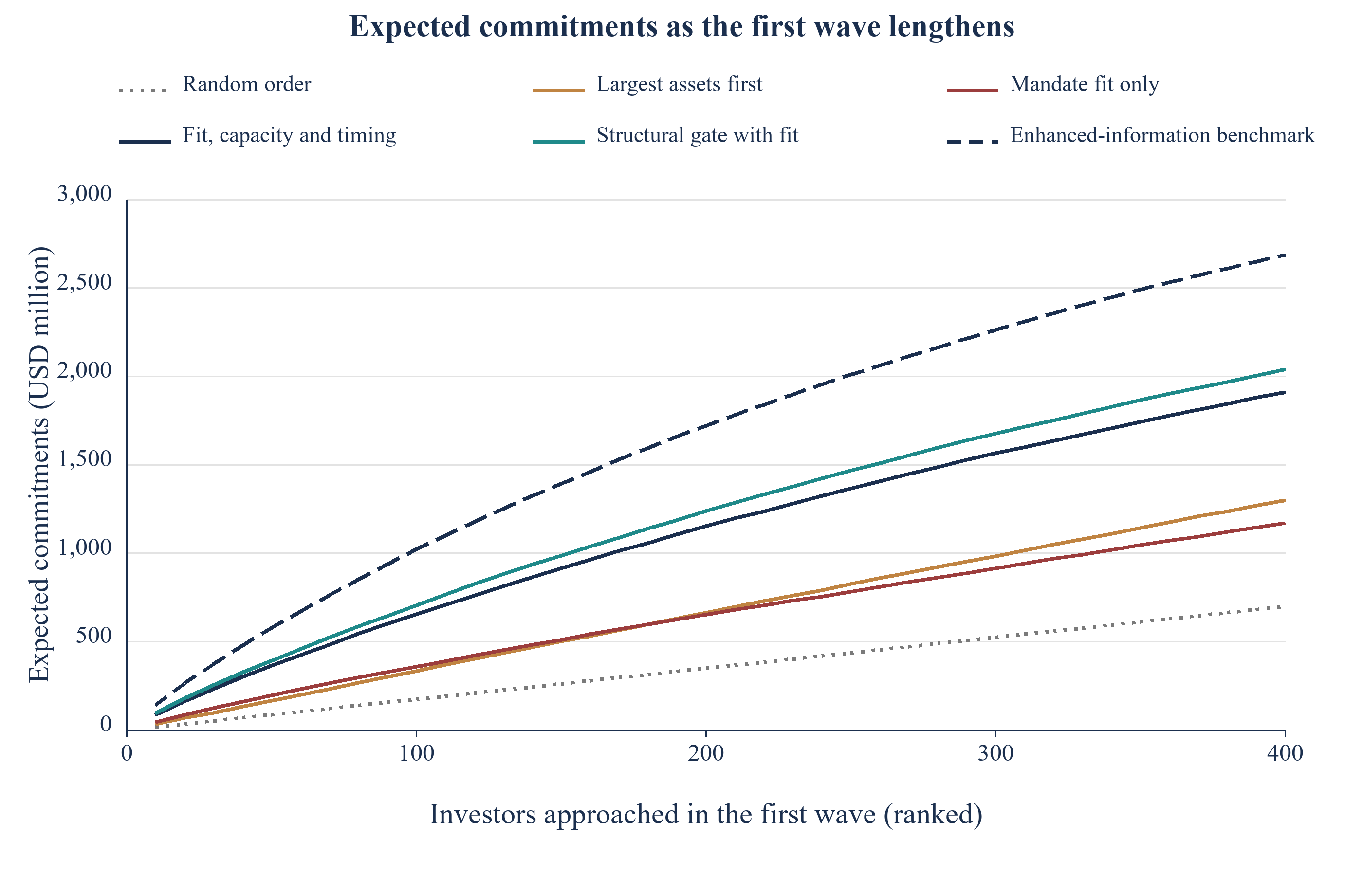
Scroll horizontally to read the figure at full size. You can also open the full-size figure.
Constructed model output under stated assumptions. Mean of 100 replications; the dashed benchmark also knows latent fit and the generated future capacity path while integrating over appetite. No observed fundraising data.
13 Incremental ranking contribution of the recorded variables
Table 6 reports two tests for each variable. The first removes it from the full score and measures lost skill. The second adds it to a score that contains only fit and measures gained skill. The two answers differ when variables carry the same information, so both are needed. Mandate fit and allocation headroom are the two variables whose removal costs measurable skill, at 0.135 and 0.123. Assets under management costs 0.023 when removed, with a spread that includes zero.
| Variable | Skill lost when removed | 10th to 90th percentile | Skill added to fit alone | 10th to 90th percentile |
|---|---|---|---|---|
| Mandate fit | 0.135 | 0.075 to 0.194 | base | not applicable |
| Allocation headroom (gap to target) | 0.123 | 0.079 to 0.180 | 0.190 | 0.116 to 0.258 |
| Assets under management | 0.023 | -0.016 to 0.063 | 0.124 | 0.053 to 0.192 |
| Budget utilisation (pacing) | 0.006 | -0.019 to 0.036 | 0.024 | -0.015 to 0.090 |
| Calendar (committee date and fiscal reset) | -0.003 | -0.039 to 0.025 | 0.108 | 0.046 to 0.174 |
| Distribution yield (recycling) | -0.004 | -0.030 to 0.013 | 0.006 | -0.030 to 0.043 |
| Unfunded commitment ratio | -0.008 | -0.037 to 0.011 | 0.026 | -0.018 to 0.080 |
MatchPoint analysis of the constructed universe. Model output under stated inputs; not an observed result. Skill is on a scale where random order is 0 and the latent ceiling is 1. Spreads are 10th to 90th percentiles across 100 replications.
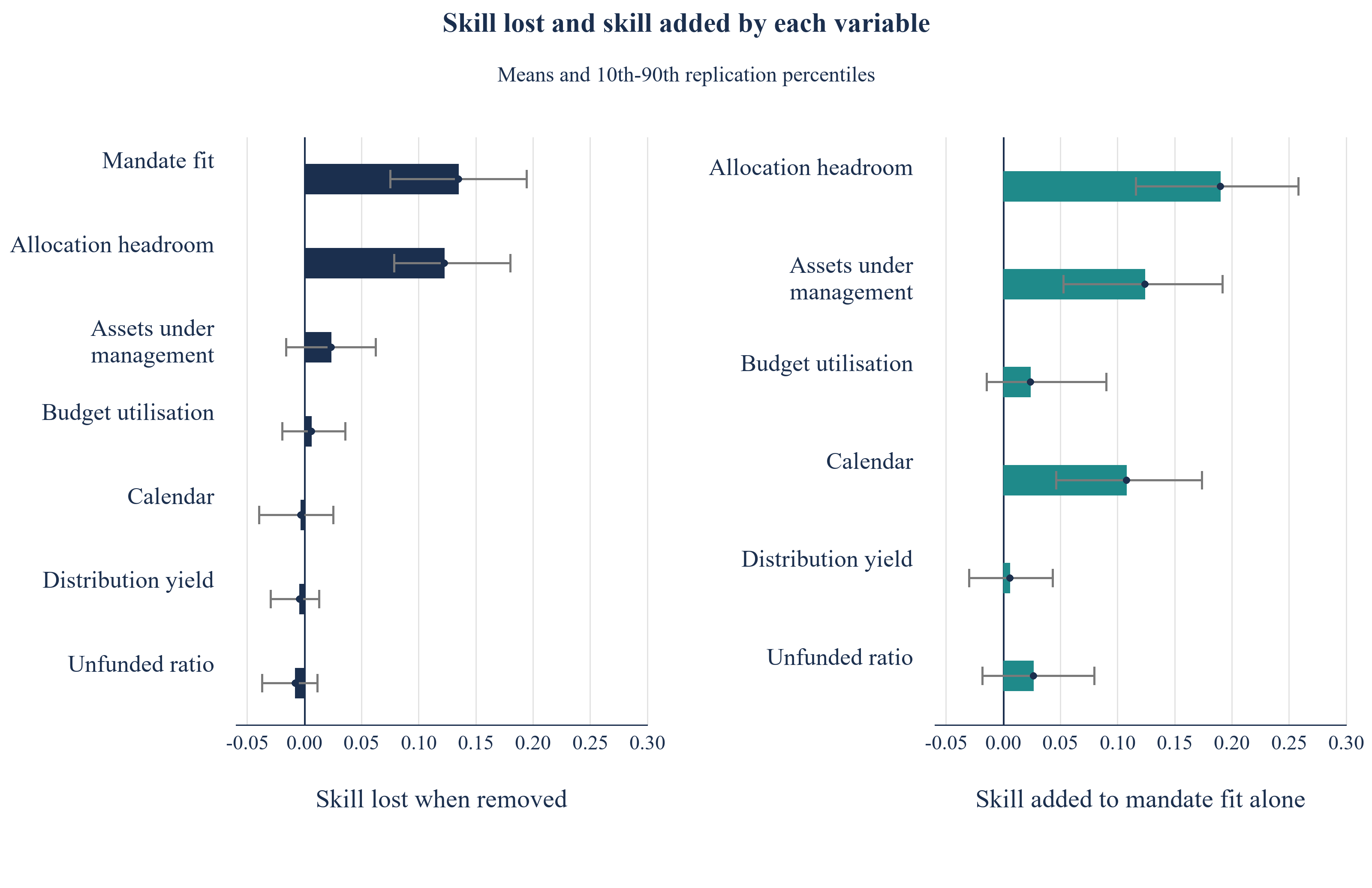
Scroll horizontally to read the figure at full size. You can also open the full-size figure.
MatchPoint analysis of the constructed universe. Model output under stated inputs; not an observed result. Bars are means over 100 replications; lines span the 10th to 90th percentile.
Calendar variables add 0.108 to fit alone in the additive model. Investor-type indicators add 0.137, and adding calendar variables after type adds -0.011, with replication percentiles -0.048 to 0.019. The average incremental ranking contribution is small after these type controls. This comparison does not identify every calendar effect as a type effect. The mechanism contains timing constraints that an additive regression may represent poorly. Section 15 examines a different decision: selecting an approach month for a fixed investor set.
Unfunded ratio, distribution yield and budget utilisation add little average skill under this generator. Their scales and observation noise are authored inputs. The 10th-to-90th replication spans for several lower-ranked variables cross zero. These spans describe repeated simulated campaigns and are not hypothesis tests for real investor populations. Correlated variables can substitute for one another in an additive score, so a small ablation contribution does not establish that an input lacks practical relevance. Section 18 reports agreement with a finite fitted-coefficient reference at different simulated cohort sizes.
14 Meetings reward fit, while commitments reward capacity and timing
Table 7 follows the same selected waves through the generated funnel. Among the operational rules compared, fit alone gives the most expected qualified meetings: 65.7 per hundred approaches, against 38.5 for random order. The full score gives 50.4 expected meetings and 26.3 expected commitments, compared with 14.4 commitments under fit alone. Largest-first gives 38.7 expected meetings and 13.4 expected commitments. The oracle uses privileged information and is reported separately. Figure 3 displays these expected counts; none is an observed campaign total.
| Ranking rule | Qualified meetings | Diligence started | Commitments | Commitments per meeting |
|---|---|---|---|---|
| Random order | 38.5 | 17.9 | 7.0 | 18% |
| Largest assets first | 38.7 | 19.3 | 13.4 | 35% |
| Mandate fit only | 65.7 | 36.5 | 14.4 | 22% |
| Fit, capacity and timing | 50.4 | 31.9 | 26.3 | 52% |
| Structural gate with fit | 58.1 | 36.7 | 28.3 | 49% |
| Latent ceiling | 73.8 | 55.7 | 54.3 | 74% |
MatchPoint analysis of the constructed universe. Model output under stated inputs; not an observed result. Expected counts per 100 approached, mean of 100 replications.
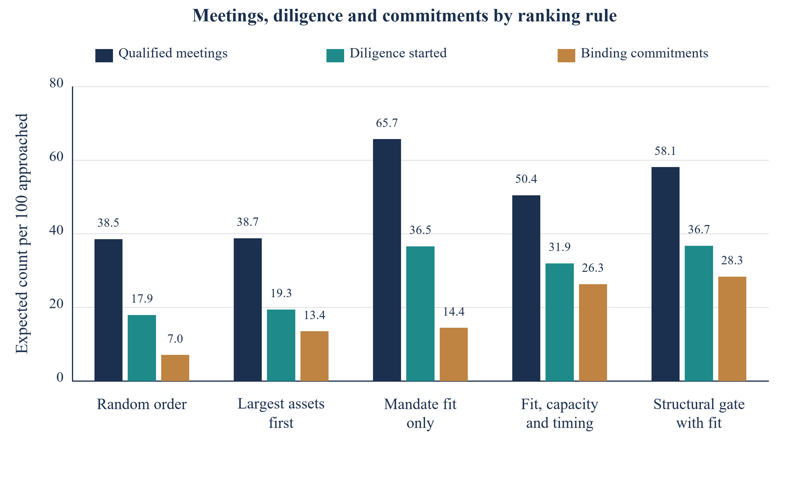
Scroll horizontally to read the figure at full size. You can also open the full-size figure.
MatchPoint analysis of the constructed universe. Model output under stated inputs; not an observed result. Expected counts per 100 investors approached, mean of 100 replications.
The funnel also shows where each rule loses investors. Fit alone sends many investors to a meeting that cannot commit in the window, and they leave at the diligence or approval stage, which consumes the team's time without producing a signature. The fitted score spends fewer meetings and loses fewer of them late, which matters when senior time is the scarce resource. Meetings are cheap to count and expensive to hold.
Expected commitments per expected meeting are 22% for fit alone, 35% for largest-first and 52% for the full score. Fit’s meeting and commitment lifts relative to random order are 1.71 and 2.05; the full score’s are 1.31 and 3.75. Under this mechanism, choosing a policy solely by expected meetings selects a different rule from choosing it by expected commitments. A prospective study would need to establish whether that distinction persists in its own investor population.
Early-stage capacity sensitivity is limited by construction. For an investor blocked at approach, the model multiplies the conditional diligence-start probability by 0.65, equivalent to a 35% relative reduction. It does not simulate an observed 35% decline rate at the meeting or explain all causes of failed diligence. The proposed study records actual stage outcomes and dates to investigate those channels without assuming them in advance.
15 Approaching each investor in a month chosen from its calendar recovers part of the timing gap
A first wave can have a planned sequence. Table 8 compares four schedules for the same 100 investors selected by the fitted score. Approaching all at launch supplies the baseline. Randomly spreading approaches over the first four months gives 0.99 times baseline expected commitments. The observed-record rule chooses each investor’s approach month from months zero through six and gives 1.01 times baseline. The perfect-information comparator uses the same feasible months and gives 1.09 times baseline. This common choice set keeps the timing comparison aligned.
| Approach plan | Expected commitments (USD m) | 10th to 90th percentile | Ratio to launch plan |
|---|---|---|---|
| Approach all at launch | 657 | 572 to 730 | 1.00 |
| Spread at random over four months | 649 | 572 to 727 | 0.99 |
| Calendar-aware month from the records | 665 | 593 to 746 | 1.01 |
| Best month with perfect knowledge | 713 | 624 to 805 | 1.09 |
MatchPoint analysis of the constructed universe. Model output under stated inputs; not an observed result. Expected commitments for the 100 investors with the highest fitted score. Spread is the 10th to 90th percentile across 100 replications.
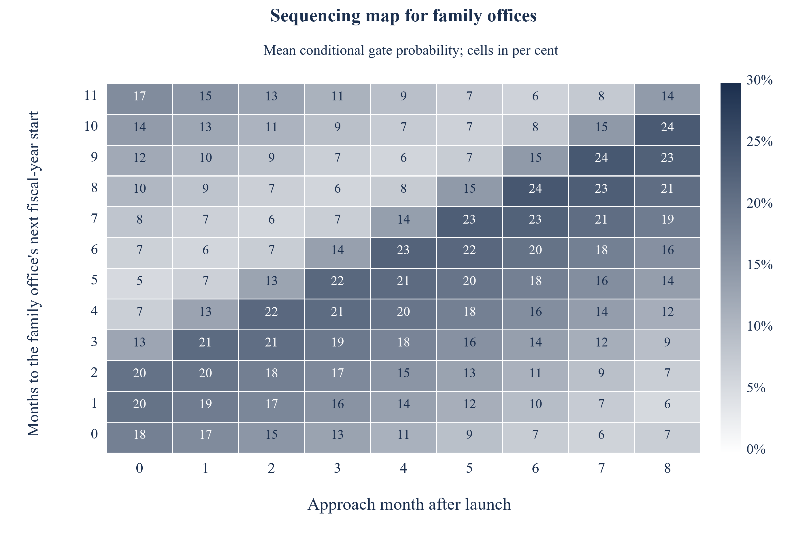
Scroll horizontally to read the figure at full size. You can also open the full-size figure.
Constructed model output under stated assumptions. Cells show mean conditional probabilities, in per cent, of passing the capacity and budget gate at a decision within the fixed twelve-month window, grouped by approach month and months to the next fiscal-year start. They do not show the share passing the separate 50% ability threshold. The descriptive grid uses months 0 through 8; both timing policies optimise over months 0 through 6.
Figure 4 shows why a mechanical stagger fails and a calendar-aware plan helps. For family offices, whose fiscal year starts in a random month, the probability of being able to commit is highest on a diagonal: it peaks near 24% when the approach falls about two months before the reset, so that a diligence of the median two months ends just after the new budget opens, and it falls to 5% when the decision lands late in the fiscal year, after the budget is largely used. Institutions with a January year start commit most often when approached in the first months, at 63% at launch against 16% when approached in month eight.
The observed-record timing rule gives 1.01 times baseline expected commitments and improves on launch in 68% of replications. Its mean gain accounts for 15% of the gap between launch and the same-feasible-set perfect-information timing benchmark. The gain is small and varies across the constructed campaigns. The selected list already has a mean conditional gate probability of 82% at launch. A live team should verify its decision dates and budgets before deferring an approach; this experiment establishes no universally better waiting rule.
16 Ranking skill and calibration under the stated stress worlds
Scores fitted on the base universe are frozen before each stress test. Each stress changes a stated part of the generating world without refitting. Table 9 reports the fitted score’s ranking skill, largest-first skill, forecast-to-reference commitment ratio, mean gate probability and mean conditional commitment probability. In the base case the top-list forecast ratio is 1.32. Figure 5 displays ranking and forecast behaviour under the specified worlds. These are comparative scenario diagnostics; the experiment does not measure an operational warning time before a real fundraising shortfall.
| World | Skill of the fitted score | Skill of largest-first | Forecast divided by conditional-reference expected commitments | Top-list mean gate probability | Average commitment probability |
|---|---|---|---|---|---|
| Base case | 0.40 | 0.13 | 1.32 | 83% | 7.0% |
| Public equities fall after the records are filed | 0.42 | 0.11 | 1.50 | 76% | 5.0% |
| Records twice as stale | 0.40 | 0.13 | 1.34 | 83% | 7.0% |
| Distributions fall by 60 per cent | 0.40 | 0.13 | 1.34 | 81% | 6.6% |
| Committees meet half as often | 0.34 | 0.14 | 1.56 | 70% | 6.3% |
| Colder appetite for the asset class | 0.36 | 0.11 | 2.26 | 83% | 3.8% |
MatchPoint analysis of the constructed universe. Model output under stated inputs; not an observed result. Mean of 60 replications. Forecast-to-conditional-reference ratio is the sum of predicted commitment probabilities over the top list divided by the sum of true probabilities.
Under the specified post-record market shock, the full score’s mean skill is 0.42 and its forecast-to-reference ratio 1.50. The capacity equation increases the simulated private-share exposure before applying the headroom floor. This can reduce expected commitment capacity without the same reduction in average ranking skill. It does not preserve every investor’s relative order. The reduced-committee and colder-appetite worlds give skills 0.34 and 0.36, with forecast ratios 1.56 and 2.26. Those comparisons are conditional scenario results.
The scenarios motivate monitoring both ranking and calibration. A forecast shortfall with relatively stable ranking can arise under a common capacity or appetite shift in this experiment. Similar aggregate patterns could have other causes in a live campaign. Investigate data quality, eligibility, follow-up, terms and unrecorded selection before changing a forecast. Largest-first skill ranges between 0.11 and 0.14 across the stated worlds. Greater record lag and reduced distributions give skills 0.40 and 0.40 under parameters that make distribution yield a relatively small input. Neither result establishes robustness to actual liquidity shocks.
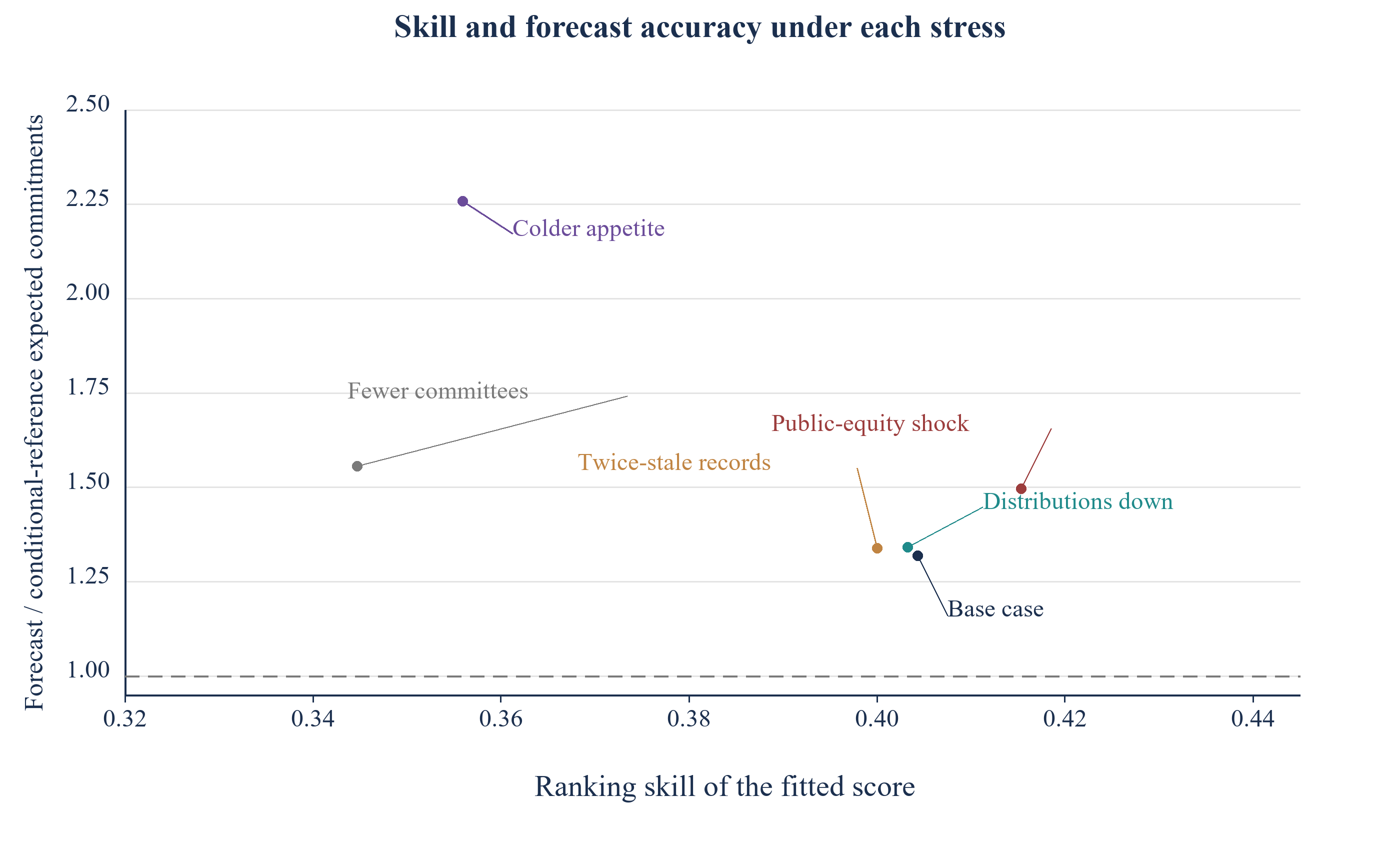
Scroll horizontally to read the figure at full size. You can also open the full-size figure.
MatchPoint analysis of the constructed universe. Model output under stated inputs; not an observed result. Mean of 60 replications per world.
17 A history selected by judgement overstates the forecast, and reweighting on the records repairs little of it
Past outreach is rarely random. A team approaches the investors it knows, and what it knows is partly appetite that no record contains. In the model, selection into the training cohort rises with appetite, fit and size. Table 10 compares four training cohorts. A random cohort of 800 gives skill 0.40 and a whole-list forecast ratio of 0.99. A judgement-selected cohort of the same size gives skill 0.40 but a ratio of 1.16, so the rate expected on the rest of the list is overstated by 16%.
| Training cohort | Skill of the fitted score | Forecast divided by reference expectation, whole list | Forecast divided by reference expectation, top list | Fit coefficient | Headroom coefficient |
|---|---|---|---|---|---|
| Random cohort of 800 | 0.40 | 0.99 | 1.34 | 0.52 | 0.89 |
| Judgement-selected cohort of 800 | 0.40 | 1.16 | 1.44 | 0.41 | 0.94 |
| Judgement-selected, reweighted on records | 0.40 | 1.15 | 1.45 | 0.42 | 0.92 |
| Random slice of 160 only | 0.34 | 1.01 | 1.74 | 0.47 | 0.79 |
MatchPoint analysis of the constructed universe. Model output under stated inputs; not an observed result. Mean of 100 replications. Coefficients are on standardised variables in the fitted commitment score.
The standard correction weights each selected investor by the inverse of its estimated probability of selection, using the variables that are recorded. Equation 4a writes the weighted log-likelihood and equation 4b the estimated weight. The weight gives more influence to investors that the team was unlikely to approach, so that the cohort resembles the whole list in its recorded variables.
Here S is the selected cohort, y_i the commitment indicator, p_i(beta) the fitted probability and x_i the recorded feature set. Reweighting reduces the constructed forecast excess from 16% to 15%, or 5% of the original excess, in this implementation. The selection rule also depends on unrecorded appetite. Estimated propensity weights based on the available features cannot remove that omitted selection channel. A random training slice of 160 has a whole-list mean forecast ratio 1.01 and skill 0.34 across replications. Random sampling does not make a finite-sample, penalised or misspecified fitted predictor unbiased. Calibration of a selected top list requires its own validation.
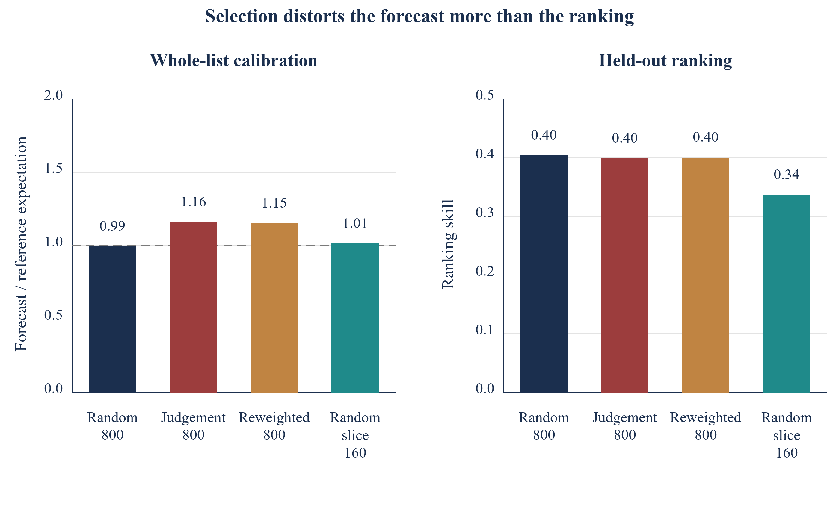
Scroll horizontally to read the figure at full size. You can also open the full-size figure.
MatchPoint analysis of the constructed universe. Model output under stated inputs; not an observed result. Mean of 100 replications.
The propensity exercise also needs a precise sampling interpretation. The selected cohort is drawn without replacement using relative weights based partly on latent appetite. A logistic propensity model fitted on recorded features estimates an inclusion pattern for that constructed sample. It does not observe appetite, and its probabilities are not the original relative drawing weights. Reweighting can change an estimate while leaving important selection differences unresolved. In a prospective study, store the actual random-inclusion probabilities at selection time. Separately record score-driven inclusion and discretionary overrides; combining these mechanisms without their probabilities prevents a transparent assessment of which population a calibration estimate represents.
18 Cohort size and agreement with the fitted reference
Table 11 compares fits on random generated cohorts of 100 to 1,600 investors. At 100 approaches, the training sample contains 7.7 commitments on average, and mean ranking skill is 0.29, with replication percentiles 0.17 to 0.39. At 800 approaches, the corresponding figures are 55.8, 0.41, 0.34 and 0.47. These are finite-simulation summaries. The top-three column compares estimated standardised-coefficient rankings with a separate finite 20,000-investor fit.
| Approached cohort | Commitments observed | Mean skill | 10th to 90th percentile | Fitted score beats largest-first | Agreement with finite fitted top-three reference |
|---|---|---|---|---|---|
| 100 | 7.7 | 0.29 | 0.17 to 0.39 | 89% | 5% |
| 200 | 14.8 | 0.35 | 0.26 to 0.45 | 99% | 19% |
| 400 | 28.2 | 0.38 | 0.31 to 0.45 | 100% | 39% |
| 800 | 55.8 | 0.41 | 0.34 to 0.47 | 100% | 67% |
| 1,600 | 111.3 | 0.42 | 0.36 to 0.47 | 100% | 88% |
MatchPoint analysis of the constructed universe. Model output under stated inputs; not an observed result. Mean of 100 replications. Top three variables are the three features with the largest standardised coefficients, compared with a fit on 20,000 investors.
At 100 and 200 training approaches, the fitted score beats largest-first in 89% and 99% of these replications. Agreement with the reference set of three largest absolute standardised coefficients is 5% at 100, 39% at 400 and 88% at 1,600. These two measurements answer different questions: ranking performance on held-out generated investors and stability relative to a chosen coefficient reference. Neither percentage supports deploying an unvalidated score on an actual investor list.
These results describe predictive performance in the authored universe. Agreement with a finite 20,000-investor fitted reference supplies the top-three feature metric; it does not identify causal drivers or establish a population truth. Replication percentiles describe variation across simulated campaigns. They are not confidence intervals for actual fundraising outcomes. A practitioner should freeze an initial model, evaluate it on prospectively collected observations, and report calibration and ranking performance separately. Changes in coefficients across waves can reflect sampling, correlations or different investor mixes as well as changed behaviour.
19 Reproduction, controls and what the experiment cannot show
Table 12 records the numerical controls actually evaluated in the private reproduction. Probability and funnel bounds, oracle ordering, committee dates, fiscal blackouts and ticket comparisons are checked explicitly. The final fit census includes the population reference and propensity models as well as the ranking fits; every recorded fit must pass the final finite-residual checks. The independent reproduction also checks the continuous-diligence integration and fixed-seed identity. Solver residuals establish a numerical condition at the returned coefficients. They do not establish identification, empirical calibration or correctness of the assumed generating mechanism.
| Control | Result |
|---|---|
| Numerical assertions and empirical validation checks | 46 passed |
| Replications, main experiment | 100 universes of 3,600 investors |
| Replications, stress worlds | 60 |
| Fits passing the final score-residual criterion | 3,122; largest score residual below 0.000001 |
| Conditional-probability oracle against every rule | At least as high in every replication |
| Random-order floor | Matches 4,000 random draws within sampling error |
| Base-rate doubling power check | Simulated power 81% at the stated size |
| Seed | Fixed; one replication re-run reproduces its scores exactly |
MatchPoint analysis of the constructed universe. Model output under stated inputs; not an observed result. Controls are asserted when the model runs.
The central limitation is circularity. Outcomes are generated from the same capacity, budget and calendar logic that the structural score uses and that the fitted score approximates. The experiment shows how a method behaves when its premise holds. It does not show that the premise holds for real investors. Real committees may weigh capacity differently, may override a budget, or may sign for reasons that no record captures. Equally, the measurement noise, lag and disclosure shares are authored, so the gap between the fitted score and the stated privileged benchmark is a property of those inputs.
What the experiment can show is the ordering of consequences. Capacity is a conjunction, meetings and commitments respond to different variables, forecast and ranking fail separately, judgement-selected history distorts the level, and small cohorts cannot rank variables. Each of these follows from structure that the primary sources make plausible, and each can be tested with the design in the next section. Where the experiment shows a large effect, such as the gap between meetings and commitments, the first test should be whether a real campaign shows the same sign. Where it shows a small effect, such as the cost of stale records, a real campaign may show a larger one, since the assumed noise is modest.
20 A consented study needs a randomised slice, timestamps and a pre-specified analysis
The unit of the proposed study is an investor and raise episode. Record the eligible universe, inclusion probability, frozen score, approach date, channel, verified source dates and each observed stage. A governance review should establish the applicable law and the basis for processing personal data before recruitment. DIFC Article 10 provides several lawful bases; consent is one. A study may adopt consent as a design requirement without describing it as the sole legal basis for every processing operation. [15]
Where consent is the basis, the DIFC law specifies consent and withdrawal requirements. Article 34 addresses objections to direct marketing, including related profiling. The ADGM official overview similarly identifies an absolute marketing-objection right. These jurisdiction-specific examples support a documented process for notices, objections and retention. The applicable regime and financial-promotion perimeter require campaign-specific review. [15, 16]
| Element | Specification | Reason |
|---|---|---|
| Unit and window | Investor and raise; twelve months from launch | Fixes the outcome clock |
| Randomised slice | Reserve 20% of approach slots for random inclusion from the full eligible, not-yet-approached universe within pre-specified strata; record nonzero inclusion probabilities | Supports calibration for targets beyond the score-selected group |
| Stratification | Type, assets band, disclosure status, fiscal-year start | Improves precision; fixed before launch |
| Timestamps | Approach, meeting, diligence, decision and signature dates | Allows time-to-event and competing-risk analysis |
| Outcomes | Meeting, diligence, binding commitment and final decline, with administrative follow-up defined separately | Separates stages |
| Sample for a 2 times lift | 298 per arm at the base rate; 635 at half of it | Power for top-ranked against randomised slice |
| Sample for a 1.5 times lift | 1,021 per arm at the base rate | Shows the cost of detecting small lifts |
| Analysis | Cause-specific hazards and cumulative incidence; pre-registered variable list | Avoids specification search |
Proposed design. Numerical sample sizes describe a separate, equal-fixed-arm, independent-Bernoulli comparison at the constructed base rate, 5% significance and 80% target power. They are not the totals for a campaign assigning 20% of slots to exploration; unequal allocation, clustering and incomplete follow-up require a separate calculation.
Random inclusion must occur before the score determines which investors receive those reserved slots. Random ordering of an already selected wave leaves selection into that wave unchanged. Define the policy estimand as expected binding commitments per eligible approach under a frozen ranked policy compared with a stated random-inclusion policy, at comparable follow-up. Record overlap, exclusions and non-compliance. Known inclusion probabilities support appropriate weighting; the evaluation must account for repeated institutions, related mandates and spillovers. Variable coefficients and ablation scores remain predictive summaries unless a separate identification design supports a causal interpretation. [13, 14]
Table 13 illustrates how rare commitments affect a balanced validation experiment. At the constructed base rate 7.0%, its equal-arm approximation gives 298 investors per arm for a doubling and 1,021 for a one-and-a-half-times rate. Only the stated base-rate doubling case is assessed by the program’s simulation check. A 20/80 operational allocation needs a different variance calculation. Clustered institutions, overlapping mandates, censoring and uncertain event rates can further change required numbers. Small campaigns should report the observations and uncertainty supported by their design and defer claims the available sample cannot distinguish.
Pre-specify follow-up before comparing policies. A target approached near the closing deadline has less time to sign than one approached at launch. Measure the operational endpoint against the common closing date and retain time since approach as a separate variable. A later signature may be commercially valuable while remaining outside the registered endpoint. Define rules for reopened episodes, overlapping raises and institutions sharing an investment committee. If the same investor appears in several mandates, observations are not independent merely because the raise identifiers differ. Variance estimates and sample-size planning should reflect that dependence, and campaign-level summaries should remain available for an audit of pooled results.
21 Report capacity and timing to the committee as a range with a discounted forecast
The committee should receive the proposed outreach policy, evidence quality and forecast uncertainty. The constructed top-list forecast ratio is 1.31, with replication percentiles 1.03 to 1.65. These are diagnostics of the model’s own selection and estimation process. They supply no universal haircut for actual fundraising. A live planning case needs prospective calibration and an explicit treatment of uncertainty in ticket size, timing, eligibility and conversion. Table 14 separates those reporting questions.
| Item | Content | How to read it |
|---|---|---|
| Ranking evidence | Skill against random order and against largest-first, with spread | Shows whether the order is better than a naive list |
| Forecast calibration | Predicted commitments, prospectively measured policy yield and uncertainty | Assesses the proposed planning estimate under an explicit validation design |
| Recorded stage losses | Observed stage and dated reason for each closed episode | Supports investigation of possible constraints; does not identify a cause by itself |
| Calendar exposure | Number of investors whose decision falls after the window | Shows the cost of late approach |
| Records quality | Share of the list with disclosed records and their age | Shows how much of the ranking rests on imputation |
| Exploration sample | Yield under the stated random-inclusion policy and comparable follow-up | Estimates a policy comparison subject to inclusion, overlap and uncertainty assumptions |
Proposed reporting pack. Thresholds are for the team to set before launch and are not derived from the model.
A committee should see the evidence behind each proposed adjustment. Report how many binding commitments were observed, the validation population, the time horizon and the uncertainty around predicted yield. A point forecast is not a statistical upper bound. A reduction based on a simulated forecast ratio is not an empirically calibrated planning case. Keep a log of excluded and deferred investors with source dates and verification status. An imputed record can support a request for evidence, while a documented legal or mandate restriction can support exclusion. Stage records help investigate bottlenecks and should not be presented as a causal attribution of failure without an appropriate design.
Verification effort can be prioritised explicitly. Identify which missing or stale record changes an investor’s rank, proposed approach month or inclusion decision under plausible alternatives. Compare the consequences of those alternatives with the time and cost of clarification. For example, a documented reset date may justify a dated follow-up, whereas an assumed reset should trigger a question before deferral. This is a proposed information-gathering rule, not a modelled revenue claim. Keep the alternatives, source evidence and decision owner in the working record so that an exclusion caused by missing information can be distinguished from an exclusion caused by a verified constraint.
22 Use data and AI to keep the records current, not to decide who is approached
The records in this paper age. Allocation weights, unfunded ratios and calendars are restated in annual or more frequent reports, and a market move can change some of them at once. Natural language tools can extract these items from annual reports, programme reviews and board papers and flag changes, which reduces the lag, although the stress cases show that lag alone costs little ranking skill under the assumed inputs. The extraction should keep the source passage and its date with every value, and a person should confirm any value that moves a ranking position by a large step.
Keep institutional records separate from personal contact records, with documented access, retention and correction processes. Maintain the score version and the source values used for each approach decision. A change in an extracted allocation or calendar should first be reconciled against the original document and its date. Any operational use of personal data requires the applicable legal review and objection process. [15, 16]
The paper fits logistic models inside a constructed experiment. It reports no model trained on observed investor outcomes and no validated accuracy for an AI extraction system. Family-office disclosure rates and missing-data behaviour are authored inputs. No reviewed family-office dataset establishes their real distribution. A practical extraction pilot should therefore evaluate field accuracy, date alignment and consequential ranking changes against independently checked source records before its outputs influence an outreach plan.
23 A decision rule for a live raise: gate on capacity, sequence on the calendar, discount the forecast
The proposed workflow begins with verified mandate eligibility and a recorded closing deadline. Next, reconcile the ticket, portfolio record, commitment obligations, approval authority and likely decision dates. Mark missing inputs and compare the proposed schedule with a simple baseline. Assess the cost of verifying uncertain records before using them as a screen. The capacity gate is an explicit modelling proposal; its operational threshold and treatment of exceptions need validation for the mandate and governing documents.
Reserve a prospective exploration sample, record every stage and compare outcomes at the agreed follow-up horizon. The fewer-meetings and greater-commitment pattern is a result under the authored mechanism. Treat it as a hypothesis for evaluation on a real list. Record a dated reason for each deferral and the next verification step. In the constructed universe, 20% of investors failing the launch approach’s gate become eligible for at least one tested later approach inside six months. The measure describes modelled eligibility, not observed investor willingness or a promised commitment.
The proposed rule is a workflow for gathering evidence and testing a decision policy. Its numerical weights require validation for the mandate, investor population and time horizon in question. A selected campaign history can contain useful information, while its omissions and selection mechanism limit which conclusions can be drawn. Combine that history with prospective observations, verified records and explicitly stated assumptions before adopting a forecast.
24 Limitations and the next decision
The experiment is constructed. Its investor types, distributions, noise levels and decision rules are authored. It contains one asset class and one ticket, a single launch month and a single window, and no competition for capacity between raises. It treats investors as independent, which ignores the information that investors share. It models fit and appetite as independent of capacity, which a real committee may not respect. It does not model fees, terms or side letters, and the records it provides are cleaner than many real ones.
The source examples cover a public pension, sovereign-investor disclosures and university endowment reports. Their transparency and accounting definitions differ. No reviewed family-office dataset supports the simulated family-office calendars or disclosure probabilities. Academic references address related fund performance, fundraising, liquidity and study-design questions. The dated 2022 CalPERS policy attachment is retained for explicitly historical discussion of target revision and policy ranges, alongside newer 2026 programme material; current authority for a transaction must be verified independently. Privacy examples are confined to the cited DIFC law and ADGM overview and do not determine the governing regime for a particular campaign.
The next decision is whether a campaign can support a pre-specified prospective evaluation. That requires an eligible-universe record, a lawful recruitment and processing plan, random inclusion where the design calls for it, and consistent outcome and follow-up definitions. Start by measuring policy yield and forecast calibration. A small list can still improve record quality and scheduling, while supporting limited conclusions about predictive superiority. The scale and uncertainty of the proposed study should be assessed before a committee relies on its eventual results.
References
- California Public Employees' Retirement System. Total Fund Investment Policy, Investment Committee agenda item 5a, attachment 3, November 2022. Marked-up draft showing tracked changes, effective date of the earlier text 13 June 2022; its private equity target was superseded by a 17 per cent target approved in March 2024. https://calpers.ca.gov/documents/202211-invest-item05a-03-a/download
- California Public Employees' Retirement System. Private Equity Annual Program Review as of 31 December 2024, Investment Committee agenda item 6c, attachment 1, 16 June 2025. Staff presentation. https://www.calpers.ca.gov/documents/202506-invest-agenda-item06c-01/download
- Meketa Investment Group. Annual Program Review, memorandum to the CalPERS Investment Committee, 16 June 2025, data as of 31 March 2025. Consultant memorandum. https://www.calpers.ca.gov/documents/202506-invest-agenda-item06c-02/download
- California Public Employees' Retirement System. Board Meetings Calendar, 2026 scheduled meetings. Web page accessed 14 October 2026. https://www.calpers.ca.gov/about/board/board-meetings/calendar
- Abu Dhabi Investment Authority. 2025 Review. Annual review, published 2026; long-term strategy portfolio ranges and private equity commentary. https://www.adia.ae/en/pr/2025/pdf/ADIA%20Annual%20Review%202025_FINAL.pdf
- Mubadala Investment Company. Strong performance by UAE portfolio drives Mubadala's growth in 2025. Press release, 9 April 2026. https://www.mubadala.com/en/news/strong-performance-by-uae-portfolio-drives-mubadalas-growth-in-2025
- Harvard Management Company. FY25 HMC Annual Report, portfolio strategy excerpt, October 2025. Two-page document. https://www.hmc.harvard.edu/wp-content/uploads/2025/10/FY25_HMC_Annual_Report.pdf
- Institutional Limited Partners Association. ILPA Principles 3.0: Fostering Transparency, Governance and Alignment of Interests for General and Limited Partners. 2019. Voluntary industry principles; later editions not checked. https://ilpa.org/wp-content/uploads/2019/06/ILPA-Principles-3.0_2019.pdf
- Robinson, D. T. and Sensoy, B. A. Cyclicality, Performance Measurement, and Cash Flow Liquidity in Private Equity. NBER Working Paper 17428, September 2011; published in the Journal of Financial Economics, 2016. Working paper version reviewed. https://nber.org/system/files/working_papers/w17428/w17428.pdf
- Barber, B. M. and Yasuda, A. Interim Fund Performance and Fundraising in Private Equity. Working paper, 29 October 2015; published in the Journal of Financial Economics, 2017. Working paper version reviewed. https://conference.nber.org/conf_papers/f82479/f82479.pdf
- Kaplan, S. N. and Schoar, A. Private Equity Performance: Returns, Persistence and Capital Flows. NBER Working Paper 9807, 2003; published in the Journal of Finance, 2005. Working paper version reviewed. https://www.nber.org/system/files/working_papers/w9807/w9807.pdf
- Luxenberg, E., Boyd, S., Kochenderfer, M. and others. Strategic Asset Allocation with Illiquid Alternatives. arXiv preprint 2207.07767, version dated 19 July 2022. Not peer reviewed. https://arxiv.org/pdf/2207.07767
- Duflo, E., Glennerster, R. and Kremer, M. Using Randomization in Development Economics Research: A Toolkit. NBER Technical Working Paper 333, December 2006. https://www.nber.org/system/files/working_papers/t0333/t0333.pdf
- Austin, P. C., Lee, D. S. and Fine, J. P. Introduction to the Analysis of Survival Data in the Presence of Competing Risks. Circulation, 2016, 133(6), PMC4741409. https://pmc.ncbi.nlm.nih.gov/articles/PMC4741409/
- Dubai International Financial Centre. Data Protection Law, DIFC Law No. 5 of 2020, consolidated July 2025. Articles 10, 12, 13 and 34. Official statutory text, accessed 18 November 2026. https://assets.difc.com/v1/media/edge/images/dubaiintern0078-difcexperie96c5-production-3253/media/project/difcexperiences/difc/difcwebsite/documents/laws--regulations/data-protection-law.pdf
- Abu Dhabi Global Market. Overview of the ADGM Data Protection Regulations 2021, brochure, May 2025. Official overview, not the regulation text. https://assets.adgm.com/download/assets/Overview+of+the+ADGM+Data+Protection+Regulations+2021+Brochure.pdf/b131764858a111efb6605e7c57113ad4
- Harvard Management Company. Message from the Chief Executive Officer, October 2026, fiscal 2026 annual report excerpt, three PDF pages. Private-equity allocation and unfunded commitments use different stated portfolio denominators. https://www.hmc.harvard.edu/wp-content/uploads/2026/10/FY26_HMC_Annual_Report.pdf
- California Public Employees' Retirement System. Private Equity Annual Program Review, Investment Committee agenda item 6c, attachment 1, 15 June 2026, 68 pages. https://www.calpers.ca.gov/documents/202606-invest-agenda-item06c-01-a/download?inline=
- Meketa Investment Group. Private equity programme review memorandum to the CalPERS Investment Committee, 15 June 2026, 11 pages; portfolio data as of 31 March 2026, subject to the valuation lags stated in the memorandum. https://www.calpers.ca.gov/documents/202606-invest-agenda-item06c-02-a/download?inline=
About the Author
Chennakeshav (CK) is a corporate finance and investment banking executive with 25+ years of global experience in deal origination, structuring and execution across M&A, growth capital and corporate strategy. He has led value-creation mandates for founders, corporates and funds — bridging the boardroom view to hands-on execution and close.
His career spans Morgan Stanley, HSBC, Lloyds Banking Group, EWEC, ADQ portfolio companies and Emirates Growth Fund, across TMT, real estate, fintech, deeptech, cleantech, infrastructure and energy. He has partnered with C-suite leaders, private equity and venture funds, sovereign wealth funds and family offices to finance complex fund raises and scale-up ventures, and has led M&A due diligence, post-merger integration and business-transformation initiatives to create value.
At Matchpoint Partners he is Managing Partner, leading the firm's corporate finance, M&A and capital-raising practice. He holds an MBA from London Business School, an engineering degree from VTU and a Master of Laws (LLM, in progress) from UCL London.
An active start-up mentor, CK mentors at Techstars, DIFC FinTech Hive, Startup Grind, Founder Institute and IN5, serves as Entrepreneur Mentor in Residence (EMiR) at London Business School, and judges the Entrepreneurship World Cup.
https://www.linkedin.com/in/ckadya/
https://www.matchpoint-partners.com/team/ck-adya.html
Disclaimer
This paper is part of a continuing series on the structure of private and alternative markets. The views expressed are the author's own. The paper is for information only, describes market structure in general terms, and does not constitute investment, legal, tax or regulatory advice or a recommendation in respect of any security, vehicle or counterparty.
